
Silverman's Mode Estimation Method Explained - adereth. I started digging into the history of mode detection after watching Aysylu Greenberg’s Strange Loop talk on benchmarking.
She pointed out that the usual benchmarking statistics fail to capture that our timings may actually be samples from multiple distributions, commonly caused by the fact that our systems are comprised of hierarchical caches. I thought it would be useful to add the detection of this to my favorite benchmarking tool, Hugo Duncan’s Criterium. Not surprisingly, Hugo had already considered this and there’s a note under the TODO section: I hadn’t heard of using kernel density estimation for multimodal distribution detection so I found the original paper, Using Kernel Density Estimates to Investigate Multimodality (Silverman, 1981).
The original paper is a dense 3 pages and my goal with this post is to restate Silverman’s method in a more accessible way. What is a mode? ModeSeekingByMedoidShifts_SheikhKhanKanade2007.pdf. Mode_detection.pdf. Proceedings/papers/v22/thiesson12/thiesson12.pdf. Distributions in Mathematica. These notes explain how to compute probabilities for common statistical distributions using Mathematica.
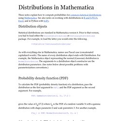
See also notes on working with distributions in R and S-PLUS, Excel, and in Python with SciPy. Distribution objects Statistical distributions are standard in Mathematica version 6. Prior to that version, you had to load either the DiscreteDistributions or ContinuousDistributions package. For example, to load the latter you would enter the following. <<Statistics`ContinuousDistributions` As with everything else in Mathematica, names use Pascal case (concatenated capitalized words). Probability density function (PDF) To calculate the PDF (probability density function) of a distribution, pass the distribution as the first argument to PDF[] and the PDF argument as the second argument. PDF[ GammaDistribution[2, 3], 17.2 ] How To Identify Patterns in Time Series Data: Time Series Analysis. Stats. Chart of distribution relationships. Probability distributions have a surprising number inter-connections.
A dashed line in the chart below indicates an approximate (limit) relationship between two distribution families. A solid line indicates an exact relationship: special case, sum, or transformation. Click on a distribution for the parameterization of that distribution. Click on an arrow for details on the relationship represented by the arrow. Follow @ProbFact on Twitter to get one probability fact per day, such as the relationships on this diagram. More mathematical diagrams The chart above is adapted from the chart originally published by Lawrence Leemis in 1986 (Relationships Among Common Univariate Distributions, American Statistician 40:143-146.) Parameterizations The precise relationships between distributions depend on parameterization. Let C(n, k) denote the binomial coefficient(n, k) and B(a, b) = Γ(a) Γ(b) / Γ(a + b). Www.pnas.org/content/early/2013/10/28/1313476110.full.pdf.
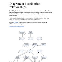
Stats 329 - Winter 2009/2010. Www.johndcook.com/Beautiful_Testing_ch10.pdf. Diagram of conjugate prior relationships. The following diagram summarizes conjugate prior relationships for a number of common sampling distributions.
Arrows point from a sampling distribution to its conjugate prior distribution. The symbol near the arrow indicates which parameter the prior is unknown. These relationships depends critically on choice of parameterization, some of which are uncommon. This page uses the parameterizations that make the relationships simplest to state, not necessarily the most common parameterizations. See footnotes below. More mathematical diagrams Click on a distribution to see its parameterization. See this page for more diagrams on this site including diagrams for probability and statistics, analysis, topology, and category theory. Parameterizations Let C(n, k) denote the binomial coefficient(n, k).
The geometric distribution has only one parameter, p, and has PMF f(x) = p (1-p)x. Random inequalities I: introduction. Many Bayesian clinical trial methods have at their core a random inequality.
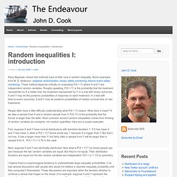
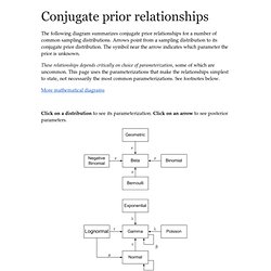
Some examples from M. D. Anderson: adaptive randomization, binary safety monitoring, time-to-event safety monitoring. These method depends critically on evaluating P(X > Y) where X and Y are independent random variables. Roughly speaking, P(X > Y) is the probability that the treatment represented by X is better than the treatment represented by Y. People often have a little difficulty understanding what P(X > Y) means. First, suppose X and Y have normal distributions with standard deviation 1. Next, suppose X and Y are identically distributed. I believe there’s a psychological tendency to underestimate large inequality probabilities. The density function for X is essentially the same as Y but shifted to the right. The image above and the numerical results mentioned in this post were produced by the Inequality Calculator software. Part II will discuss analytically evaluating random inequalities.
Inferential Statistics.