Forecasting

Forecasting: principles and practice. Welcome to our online textbook on forecasting.

This textbook is intended to provide a comprehensive introduction to forecasting methods and to present enough information about each method for readers to be able to use them sensibly. We don’t attempt to give a thorough discussion of the theoretical details behind each method, although the references at the end of each chapter will fill in many of those details. 13 Resources. Time series - AR(1) selection using sample ACF-PACF. Forecasting within limits. Forecasting within limits It is com­mon to want fore­casts to be pos­i­tive, or to require them to be within some spec­i­fied range .

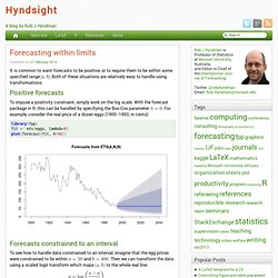
Both of these sit­u­a­tions are rel­a­tively easy to han­dle using transformations. Pos­i­tive forecasts To impose a pos­i­tiv­ity con­straint, sim­ply work on the log scale. . Fore­casts con­strained to an interval. Interpreting noise. When watch­ing the TV news, or read­ing news­pa­per com­men­tary, I am fre­quently amazed at the attempts peo­ple make to inter­pret ran­dom noise.

For exam­ple, the lat­est tiny fluc­tu­a­tion in the share price of a major com­pany is attrib­uted to the CEO being ill. When the exchange rate goes up, the TV finance com­men­ta­tor con­fi­dently announces that it is a reac­tion to Chi­nese build­ing con­tracts. No one ever says “The unem­ploy­ment rate has dropped by 0.1% for no appar­ent reason.” What is going on here is that the com­men­ta­tors are assum­ing we live in a noise-​​free world. They imag­ine that every­thing is explic­a­ble, you just have to find the expla­na­tion. The finance news Every night on the nightly TV news bul­letins, a sup­posed expert will go through the changes in share prices, stock prices indexes, cur­rency rates, and eco­nomic indi­ca­tors, from the past 24 hours.

Errors on percentage errors. The MAPE (mean absolute per­cent­age error) is a pop­u­lar mea­sure for fore­cast accu­racy and is defined as where denotes an obser­va­tion and denotes its fore­cast, and the mean is taken over Arm­strong (1985, p.348) was the first (to my knowl­edge) to point out the asym­me­try of the MAPE say­ing that “it has a bias favor­ing esti­mates that are below the actual val­ues”.

A few years later, Arm­strong and Col­lopy (1992) argued that the MAPE “puts a heav­ier penalty on fore­casts that exceed the actual than those that are less than the actual”. And. Modelling seasonal data with GAMs. In previous posts I have looked at how generalized additive models (GAMs) can be used to model non-linear trends in time series data.

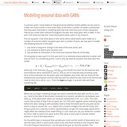
At the time a number of readers commented that they were interested in modelling data that had more than just a trend component; how do you model data collected throughout the year over many years with a GAM? In this post I will show one way that I have found particularly useful in my research. First an equation. Monthly seasonality. I regularly get asked why I don’t consider monthly seasonality in my models for daily or sub-daily time series.

For example, this recent comment on my post on seasonal periods, or this comment on my post on daily data. The fact is, I’ve never seen a time series with monthly seasonality, although that does not mean it does not exist. Rmnppt/FruitAndVeg - HTML - GitHub. Monitoring Count Time Series in R: Aberration Detection in Public Health Surveillance. Why time series forecasts prediction intervals aren't as good as we'd hope.

Five different sources of error When it comes to time series forecasts from a statistical model we have five sources of error: Random individual errors Random estimates of parameters (eg the coefficients for each autoregressive term) Uncertain meta-parameters (eg number of autoregressive terms) Unsure if the model was right for the historical data Even given #4, unsure if the model will continue to be right.

Prophet. Rolling Origins and Fama French. By Jonathan Regenstein Today, we continue our work on sampling so that we can run models on subsets of our data and then test the accuracy of the models on data not included in those subsets.

In the machine learning prediction world, these two data sets are often called training data and testing data, but we’re not going to do any machine learning prediction today. We’ll stay with our good’ol Fama French regression models for the reasons explained last time: the goal is to explore a new method of sampling our data and I prefer to do that in the context of a familiar model and data set. In 2019, we’ll start expanding our horizons to different models and data, but for today it’s more of a tools exploration.

Cross-validation for time series forecast. Time series cross-validation is important part of the toolkit for good evaluation of forecasting models. forecast::tsCV makes it straightforward to implement, even with different combinations of explanatory regressors in the different candidate models for evaluation.

Suprious correlation between time series is a well documented and mocked problem, with Tyler Vigen’s educational website on the topic (“per capita cheese consumption correlated with number of people dying by becoming entangled in their bedsheets”) even spawning a whole book of humourous examples. Identifying genuinely-correlated series can be immensely helpful for time series forecasting. Forecasting is hard, and experience generally shows that complex causal models don’t do as well as much simpler methods. However, a well chosen small set of “x regressors” can improve forecasting performance in many situations. Time series cross validation of effective reproduction number nowcasts. For a few weeks now I’ve been publishing estimates of the time-varying effective reproduction number for Covid-19 in Victoria (and as bonuses, NSW and Australia as a whole).

Reproduction number is the average number of people each infected person infects in turn. My modelling includes nowcasts up to “today” of that number (and forecasts for another 14 days ahead), a risky enterprise because the evidence of today’s number of infections is obviously only going to turn up in 7-14 days time, after incubation, presentation, testing and making its way onto the official statistics. At the time of writing, those estimates look like this: It’s been interesting watching the estimates of reproduction number change as new data comes in each morning, not least because of a personal interest (as a Melbourne-dweller) in the numbers coming down as quickly as possible.

The recent outbreak here has come under control and incidence has rapidly declined. Time series intervention analysis with fuel prices. A couple of months ago I blogged about consumer spending on vehicle fuel by income. The impetus for that post was the introduction on 1 July 2018 of an 11.5 cent per litre “regional fuel tax” in Auckland. One vehement critic of the levy, largely on the grounds of its impact on the poor, has been Sam Warburton (@Economissive on Twitter) of the New Zealand Initiative. Since early May 2018 (ie seven weeks before the fuel levy began), Sam has been collecting fuel prices from pricewatch.co.nz, and he recently made the data available.

One of the issues of controversy about a levy like this is whether it will lead to “price spreading” - fuel companies absorbing some of the extra tax in Auckland and increasing prices in other regions. SimITS. Detecting time series outliers. The tsoutliers() function in the forecast package for R is useful for identifying anomalies in a time series. However, it is not properly documented anywhere.

This post is intended to fill that gap. The function began as an answer on CrossValidated and was later added to the forecast package because I thought it might be useful to other people. It has since been updated and made more reliable. The procedure decomposes the time series into trend, seasonal and remainder components: yt=Tt+St+Rt. For data observed more frequently than annually, we use a robust approach to estimate Tt and St by first applying the MSTL method to the data.

Tidy forecasting in R. The fable package for doing tidy forecasting in R is now on CRAN. Like tsibble and feasts, it is also part of the tidyverts family of packages for analysing, modelling and forecasting many related time series (stored as tsibbles). For a brief introduction to tsibbles, see this post from last month. Here we will forecast Australian tourism data by state/region and purpose.

Fable: Tidy forecasting in R. Reintroducing tsibble: data tools that melt the clock. Reintroducing tsibble: data tools that melt the clock Preface I have introduced tsibble before in comparison with another package. Now I’d like to reintroduce tsibble (bold for package) to you and highlight the role tsibble (italic for data structure) plays in tidy time series analysis. The development of the tsibble package has been taking place since July 2017, and v0.6.2 has landed on CRAN in mid-December.

Yup, there have been 14 CRAN releases since the initial release, and it has evolved substantially. Motivation. Time series graphics using feasts. This is the second post on the new tidyverts packages for tidy time series analysis. The previous post is here. For users migrating from the forecast package, it might be useful to see how to get similar graphics to those they are used to. The forecast package is built for ts objects, while the feasts package provides features, statistics and graphics for tsibbles.

Tidyrisk - Making Quant Risk Tidy. Cleaning Anomalies to Reduce Forecast Error by 9% with anomalize. Written by Matt Dancho on September 30, 2019 In this tutorial, we’ll show how we used clean_anomalies() from the anomalize package to reduce forecast error by 9%. R Packages Covered: Introducing Modeltime: Tidy Time Series Forecasting using Tidymodels. Forecasting the next decade in the stock market using time series models. This post will introduce one way of forecasting the stock index returns on the US market. Typically, single measures such as CAPE have been used to do this, but they lack accuracy compared to using many variables and can also have different relationships with returns on different markets.