
Too crude to be true? The key to programming is being lazy; it has actually been called a virtue by some.

When I discovered the update() function it blew me away. Within short I had created a monster based upon this tiny function, allowing quick and easy output of regression tables that contain crude and adjusted estimates. In this post I’ll show you how to tame the printCrudeAndAdjusted() function in my Gmisc-package and show a little behind the scenes. Although not always present I think a regression table that shows both the crude and adjusted estimates conveys important information.
The crude is also referred to as un-adjusted and if this sharply drops in the adjusted model we can suspect that there is a strong confounder that steals some of the effect that this variable has. A simple walk-through We will start with basic usage of the function. Showing results from Cox PH Models in R with simPH. Update 2 February 2014: A new version of simPH (Version 1.0) will soon be available for download from CRAN.

It allows you to plot using points, ribbons, and (new) lines. See the updated package description paper for examples. Note that the ribbons argument will no longer work as in the examples below. Please use type = 'ribbons' (or 'points' or 'lines'). Effectively showing estimates and uncertainty from Cox Proportional Hazard (PH) models, especially for interactive and non-linear effects, can be challenging with currently available software. So, I’ve been putting together the simPH R package to hopefully make it easier to show results from Cox PH models. Here I want to give an overview of how to use simPH. General Steps There are three steps to use simPH: A Few Examples Here are some basic examples that illustrate the process and key syntax. Linear effects Let’s look at a simple example with a linear non-interactive effect. Notice that the argument spin = TRUE. Interactions. Survival - Which model should I use for Cox proportional hazards with paired data.
Cluster() or frailty() in coxph. Good looking survival curves – ‘ggsurv’ function. This is a guest post by Edwin Thoen Currently I am doing my master thesis on multi-state models.
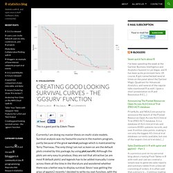
Survival analysis was my favourite course in the masters program, partly because of the great survival package which is maintained by Terry Therneau. The only thing I am not so keen on are the default plots created by this package, by using plot.survfit. Although the plots are very easy to produce, they are not that attractive (as are most R default plots) and legends has to be added manually. I come across them all the time in the literature and wondered whether there was a better way to display survival.
Once the function is loaded, we can get going, we use the lung data set from the survival package for illustration. Censored observations are denoted by red crosses, by default a confidence interval is plotted and the axes are labeled. The multi-stratum curves are by default of different colors, the standard ggplot colours. Coxph and loglik converged before variable X. R - How to extract values from survfit object. Dealing with non-proportional hazards in R. Since I’m frequently working with large datasets and survival data I often find that the proportional hazards assumption for the Cox regressions doesn’t hold.

In my most recent study on cardiovascular deaths after total hip arthroplasty the coefficient was close to zero when looking at the period between 5 and 21 years after surgery. Grambsch and Thernau’s test for non-proportionality hinted though of a problem and as I explored it there was a clear correlation between mortality and hip arthroplasty surgery. The effect increased over time, just as we had originally thought, see below figure.
Timedep. Survival Analysis with R · R Views. By Joseph Rickert With roots dating back to at least 1662 when John Graunt, a London merchant, published an extensive set of inferences based on mortality records, survival analysis is one of the oldest subfields of Statistics [1].

Basic life-table methods, including techniques for dealing with censored data, were discovered before 1700 [2], and in the early eighteenth century, the old masters - de Moivre working on annuities, and Daniel Bernoulli studying competing risks for the analysis of smallpox inoculation - developed the modern foundations of the field [2]. Today, survival analysis models are important in Engineering, Insurance, Marketing, Medicine, and many more application areas. So, it is not surprising that R should be rich in survival analysis functions. CRAN’s Survival Analysis Task View, a curated list of the best relevant R survival analysis packages and functions, is indeed formidable. Interpreting hazard ratios. Philip Sedgwick, reader in medical statistics and medical education, Katherine Joekes, senior lecturer in clinical communicationAuthor affiliationsCorrespondence to: P Sedgwick p.sedgwick@sgul.ac.uk The impact of isoniazid prophylaxis on mortality and tuberculosis in children with HIV was investigated using a double blind placebo controlled trial.
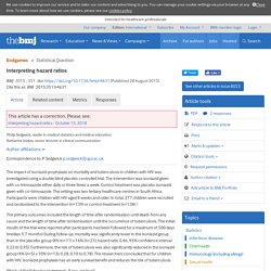
The intervention was isoniazid given with co-trimoxazole either daily or three times a week. Control treatment was placebo isoniazid given with co-trimoxazole. The setting was two tertiary healthcare centres in South Africa. Participants were children with HIV aged 8 weeks and older. On the Interpretation of the Hazard Ratio and Communication of Survival Benefit.