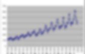
Durbin-Watson test. De-seasonality/de-trend. Autocorrelograms. A Simple Time Series Analysis Of The S&P 500 Index. In this blog post we'll examine some common techniques used in time series analysis by applying them to a data set containing daily closing values for the S&P 500 stock market index from 1950 up to present day.
The objective is to explore some of the basic ideas and concepts from time series analysis, and observe their effects when applied to a real world data set. Although it's not possible to actually predict changes in the index using these techniques, the ideas presented here could theoretically be used as part of a larger strategy involving many additional variables to conduct a regression or machine learning effort.
8.1 Linear Regression Models with Autoregressive Errors. Printer-friendly version When we do regressions using time series variables, it is common for the errors (residuals) to have a time series structure.
This violates the usual assumption of independent errors made in ordinary least squares regression. The consequence is that the estimates of coefficients and their standard errors will be wrong if the time series structure of the errors is ignored. It is possible, though, to adjust estimated regression coefficients and standard errors when the errors have an AR structure.
More generally, we will be able to make adjustments when the errors have a general ARIMA structure. The Regression Model with AR Errors Suppose that yt and xt are time series variables. Yt=β0+β1xt+ϵt with ϵt=ϕ1ϵt−1+ϕ2ϵt−2+⋯+wt, and wt∼iidN(0,σ2). If we let Φ(B)=1−ϕ1B−ϕ2B2−⋯, then we can write the AR model for the errors as Φ(B)ϵt=wt. If we assume that an inverse operator, Φ−1(B), exists, then ϵt=Φ−1(B)wt. So, the model can be written yt=β0+β1xt+Φ−1(B)wt, 1. 2. 3. Additional Comment. A Complete Tutorial on Time Series Modeling in R. Introduction ‘Time’ is the most important factor which ensures success in a business.
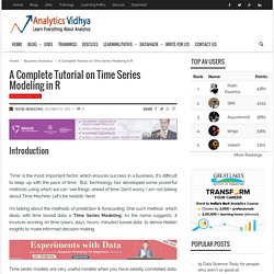
It’s difficult to keep up with the pace of time. But, technology has developed some powerful methods using which we can ‘see things’ ahead of time. Don’t worry, I am not talking about Time Machine. Let’s be realistic here! I’m talking about the methods of prediction & forecasting. Time series models are very useful models when you have serially correlated data. Complete guide to create a Time Series Forecast (with Codes in Python) Time Series (referred as TS from now) is considered to be one of the less known skills in the analytics space (Even I had little clue about it a couple of days back).
But as you know our inaugural Mini Hackathon is based on it, I set myself on a journey to learn the basic steps for solving a Time Series problem and here I am sharing the same with you. These will definitely help you get a decent model in our hackathon today. Before going through this article, I highly recommend reading A Complete Tutorial on Time Series Modeling in R, which is like a prequel to this article. It focuses on fundamental concepts and is based on R and I will focus on using these concepts in solving a problem end-to-end along with codes in Python. Many resources exist for TS in R but very few are there for Python so I’ll be using Python in this article.
Out journey would go through the following steps: What makes Time Series Special? It is time dependent. Let’s understand the arguments one by one: data.index. Forecasting - How to "undifference" a time series variable. Statistical forecasting: notes on regression and time series analysis. Robert Nau Fuqua School of Business Duke University Tweet This web site contains notes and materials for an advanced elective course on statistical forecasting that is taught at the Fuqua School of Business, Duke University.
04 09gon. Parra econometria aplicada ii5. Creation of model of SARIMA by means of Python+R — IT daily blog, news, magazine, technologies. 2 years, 4 months ago Introduction Good afternoon, dear readers.
After writing of the previous post about the analysis of time series on Python, I deciding to correct remarks who specif in comments, but at them correction I facing with a row of problems, for example at creation of seasonal model of ARIMA since similar function and a packet of statsmodels I doing not find. As a result I deciding to use for this function from R, and searches le me to library of rpy2 which pozvolyaetispolzovat to function from libraries of the mention language.
At many to arise the question «what for it it could are necessary?» Setting and adjustments of Rpy2 To start operation it are necessary ustanovt to rpy2. Pip install rpy2 It are necessary to mark that, the install language of R are necessary for operation of the g library. Beginning of operation So, if you worked in IPython Notebook, it are necessary to add the instruction: %load_ext rmagic Preliminary data analysis w_log = log(w) w_log.plot(figsize=(12,6))
SeriesUNIV MIO MP.