
Quantum gauge theory. Older approaches to quantization for Abelian models use the Gupta-Bleuler formalism with a "semi-Hilbert space" with an indefinite sesquilinear form.
However, it is much more elegant to just work with the quotient space of vector field configurations by gauge transformations. An alternative approach using lattice approximations is covered in (Wick rotated) lattice gauge theory. Common integrals in quantum field theory. There are common integrals in quantum field theory that appear repeatedly.[1] These integrals are all variations and generalizations of gaussian integrals to the complex plane and to multiple dimensions.
Other integrals can be approximated by versions of the gaussian integral. Fourier integrals are also considered. Wigner's theorem. Wigner's theorem, proved by Eugene Wigner in 1931,[1] is a cornerstone of the mathematical formulation of quantum mechanics.
The theorem specifies how physical symmetries such as rotations, translations, and CPT act on the Hilbert space of states. According to the theorem, any symmetry acts as a unitary or antiunitary transformation in the Hilbert space. More precisely, it states that a surjective (not necessarily linear) map. Invariance mechanics.
The invariant quantities made from the input and output states of a system are the only quantities needed to give a probability amplitude to a given system.
This is what is meant by the system obeying a symmetry. Since all the quantities involved are relative quantities, invariance mechanics can be thought of as taking relativity theory to its natural limit. Invariance mechanics has strong links with loop quantum gravity in which the invariant quantities are based on angular momentum. In invariance mechanics, space and time come secondary to the invariants and are seen as useful concepts that emerge only in the large scale limit.
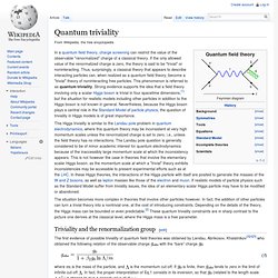
Feynman rules[edit] Scalar particles[edit] Einstein–Maxwell–Dirac equations. Einstein–Maxwell–Dirac equations (EMD) are related to quantum field theory.
The current Big Bang Model is a quantum field theory in a curved spacetime. Unfortunately, no such theory is mathematically well-defined; in spite of this, theoreticians claim to extract information from this hypothetical theory. On the other hand, the super-classical limit of the not mathematically well-defined QED in a curved spacetime is the mathematically well-defined Einstein–Maxwell–Dirac system. (One could get a similar system for the standard model.) As a super theory, EMD violates the positivity condition in the Penrose–Hawking singularity theorems. The Einstein–Yang–Mills–Dirac Equations provide an alternative approach to a Cyclic Universe which Penrose has recently been advocating. One way of trying to construct a rigorous QED and beyond is to attempt to apply the deformation quantization program to MD, and more generally, EMD.
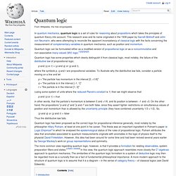
Program for SCESM[edit] Path integral formulation. Mathematically equivalent formulations of quantum mechanics. Quantum triviality. In a quantum field theory, charge screening can restrict the value of the observable "renormalized" charge of a classical theory.
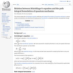
If the only allowed value of the renormalized charge is zero, the theory is said to be "trivial" or noninteracting. Thus, surprisingly, a classical theory that appears to describe interacting particles can, when realized as a quantum field theory, become a "trivial" theory of noninteracting free particles. This phenomenon is referred to as quantum triviality. Quantum logic. Quantum logic can be formulated either as a modified version of propositional logic or as a noncommutative and non-associative many-valued (MV) logic.[1][2][3][4][5] Quantum logic has some properties which clearly distinguish it from classical logic, most notably, the failure of the distributive law of propositional logic: p and (q or r) = (p and q) or (p and r), where the symbols p, q and r are propositional variables.
To illustrate why the distributive law fails, consider a particle moving on a line and let. Relation between Schrödinger's equation and the path integral formulation of quantum mechanics. Background[edit] Schrödinger's equation[edit] Schrödinger's equation, in bra–ket notation, is where.
Mathematical formulation of quantum mechanics. Theoretical and experimental justification for the Schrödinger equation. The theoretical and experimental justification for the Schrödinger equation motivates the discovery of the Schrödinger equation, the equation that describes the dynamics of nonrelativistic particles.
The motivation uses photons, which are relativistic particles with dynamics determined by Maxwell's equations, as an analogue for all types of particles. This article is at a postgraduate level. For a more general introduction to the topic see Introduction to quantum mechanics. Classical electromagnetic waves[edit] Schwinger–Dyson equation. The Schwinger–Dyson equations (SDEs), also known as the Dyson–Schwinger equations, named after Julian Schwinger and Freeman Dyson, are general relations between Green functions in quantum field theories (QFTs).
They are also referred to as the Euler–Lagrange equations of quantum field theories, since they are the equations of motion of the corresponding Green's function. They form a set of infinitely many functional differential equations, all coupled to each other, sometimes referred to as the infinite tower of SDEs. In his paper "The S-Matrix in Quantum electrodynamics",[1] Dyson derived relations between different S-matrix elements, or more specific "one-particle Green's functions", in quantum electrodynamics, by summing up infinitely many Feynman diagrams, thus working in a perturbative approach.
Spherical basis. "Spherical tensor" redirects to here. For the concept related to operators see tensor operator. While spherical polar coordinates are one orthogonal coordinate system for expressing vectors and tensors using polar and azimuthal angles and radial distance, the spherical basis are constructed from the standard basis and use complex numbers. Spherical basis in three dimensions[edit] A vector A in 3d Euclidean space ℝ3 can be expressed in the familiar Cartesian coordinate system in the standard basis ex, ey, ez, and coordinates Ax, Ay, Az: Basis definition[edit] In the spherical bases denoted e+, e−, e0, and associated coordinates with respect to this basis, denoted A+, A−, A0, the vector A is:
Ward–Takahashi identity. The Ward–Takahashi identity of quantum electrodynamics was originally used by John Clive Ward and Yasushi Takahashi to relate the wave function renormalization of the electron to its vertex renormalization factor F1(0), guaranteeing the cancellation of the ultraviolet divergence to all orders of perturbation theory. Later uses include the extension of the proof of Goldstone's theorem to all orders of perturbation theory. The Ward–Takahashi identity is a quantum version of the classical Noether's theorem, and any symmetries in a quantum field theory can lead to an equation of motion for correlation functions. This generalized sense should be distinguished when reading literature, such as Michael Peskin and Daniel Schroeder's textbook, An Introduction to Quantum Field Theory (see references), from the original sense of the Ward identity. Phase space formulation. The theory was fully detailed by Hip Groenewold in 1946 in his PhD thesis,[1] with significant parallel contributions by Joe Moyal,[2] each building off earlier ideas by Hermann Weyl[3] and Eugene Wigner.[4] The chief advantage of the phase space formulation is that it makes quantum mechanics appear as similar to Hamiltonian mechanics as possible by avoiding the operator formalism, thereby "'freeing' the quantization of the 'burden' of the Hilbert space.
"[5] This formulation is statistical in nature and offers logical connections between quantum mechanics and classical statistical mechanics, enabling a natural comparison between the two (cf. classical limit). Quantum mechanics in phase space is often favored in certain quantum optics applications (see optical phase space), or in the study of decoherence and a range of specialized technical problems, though otherwise the formalism is less commonly employed in practical situations.[6] Phase space distribution[edit] Star product[edit] or etc.) Angular momentum diagrams (quantum mechanics) In quantum mechanics and its applications to quantum many-particle systems, notably quantum chemistry, angular momentum diagrams, or more accurately from a mathematical viewpoint angular momentum graphs, are a diagrammatic method for representing angular momentum quantum states of a quantum system allowing calculations to be done symbolically.
More specifically, the arrows encode angular momentum states in bra–ket notation and include the abstract nature of the state, such as tensor products and transformation rules. They were developed primarily by Adolfas Jucys in the twentieth century. The quantum state vector of a single particle with total angular momentum quantum number j and total magnetic quantum number m = j, j − 1, ..., , −j + 1, −j, is denoted as a ket |j, m⟩. Schrödinger equation. Bloch sphere. Bloch sphere. Quantum geometry. In theoretical physics, quantum geometry is the set of new mathematical concepts generalizing the concepts of geometry whose understanding is necessary to describe the physical phenomena at very short distance scales (comparable to Planck length).
At these distances, quantum mechanics has a profound effect on physics. List of quantum-mechanical systems with analytical solutions. Fractional quantum mechanics.