SI Units. Maths. Specialized - Math. Math. ExamSolutions. Cabri Express - the all-in-one math app. Practice Vector Calculus. Math2.org. WebMath - Solve Your Math Problem. High School Resources. Find Integrals and Antiderivatives! Online Derivative Calculator. Equations solver - GetEasySolution.com. Variable on One Side Solving Two-Step Equations - WorksheetWorks.com. Algebrarules.com: The Most Useful Rules of Basic Algebra, Free & Searchable. Online maths practice. Videos and Worksheets. 2D shapes: names Video 1 Practice Questions Textbook Exercise 2D shapes: quadrilaterals Video 2 Practice Questions Textbook Exercise 3D shapes: names Video 3 Practice Questions Textbook Exercise 3D shapes: nets Video 4 Practice Questions Textbook Exercise 3D shapes: vertices, edges, faces Video 5 Practice Questions Textbook Exercise.

Basic Differentiation Tutorial. Differentiation The process of finding the gradient or slope of a function is the differentiation.
We used to find the gradient of a straight line, just by dividing the change in 'y' by change in 'x', in a certain range of values. However, when it comes to a curve, it is not easy to find the gradient or slope as the very thing we want to measure, keeps changing from point to point. we have to draw tangents at all those points and then find the gradients individually. The following animation illustrates just that.
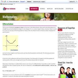
If we stick to this method we will have to draw hundreds, if not thousands, of tangents to find the gradient at various points of the curve; enough work to put off someone doing maths for decades! Good news is that there is a method that comes to our rescue. If y = xn then dy/dx = nxn-1 That means, if a curve is in the form of y = xn , its gradient at any point is given by nxn-1 . E.g. y = x2 - 2x So, dy/dx = 2x -2 E.g.1 Differentiate the following: E.g.2 Equations of tangents to a curve. Understanding Exponents (Why does 0^0 = 1?) We’re taught that exponents are repeated multiplication.
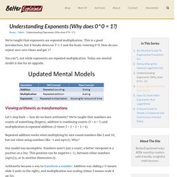
This is a good introduction, but it breaks down on 3^1.5 and the brain-twisting 0^0. How do you repeat zero zero times and get 1? You can’t, not while exponents are repeated multiplication. Today our mental model is due for an upgrade. Viewing arithmetic as transformations Let’s step back — how do we learn arithmetic? Approaches that try to avoid memorization. Algebra 1 Math Course. GeoGebra Calculus Applets. Didaxy. Exploring Precalculus. Integral Calculator - Symbolab. SineRider - A Game of Numerical Sledding. Desmos Graphing Calculator. Real World Examples of Quadratic Equations. An example of a Quadratic Equation: Quadratic equations pop up in many real world situations!
Here we have collected some examples for you, and solve each using different methods: Each example follows three general stages: Take the real world description and make some equations Solve! Use your common sense to interpret the results Ignoring air resistance, we can work out its height by adding up these three things: Add them up and the height h at any time t is: h = 3 + 14t - 5t2 And the ball will hit the ground when the height is zero: 3 + 14t - 5t2 = 0 Which is a Quadratic Equation ! -5t2 + 14t + 3 = 0 Let us solve it ... There are many ways to solve it, here we will use the factoring method: The "t = −0.2" is a negative time, impossible in our case. Exploring Precalculus. Friendly lessons for lasting insight. Example 1: The Natural Base.
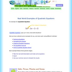
Plotted below are two familiar exponential functions: and On the interval shown, we see that 2x begins with a slight head start in value, but 3x quickly outgrows it, overtaking 2x at We also see that the larger the values of each function, the faster they grow.
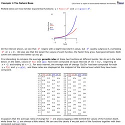
Said geometrically: Both curves are steeper the further up you go. It is interesting to compare the average growth rates of these two functions at different points. We do so in the table below. In the table, values of f(x) and g(x) have been computed at equal intervals of beginning at and ending at For each interval, the average rate of change Dy/Dx has been computed for both and and these rates are displayed at the midpoint of the interval over which they have been computed. It appears that the average rates of change for f are always lagging a little behind the values of the function itself, while those for g are always a little ahead.