
Recommended for beginners: the How-To Videos. Rel: Z transform to Laplace.
Z transform. Zeta function regularization. Definition[edit] There are several different summation methods called zeta function regularization for defining the sum of a possibly divergent series a1 + a2 + ....
One method is to define its zeta regularized sum to be ζA(−1) if this is defined, where the zeta function is defined for Re(s) large by if this sum converges, and by analytic continuation elsewhere. In the case when an = n, the zeta function is the ordinary Riemann zeta function, and this method was used by Euler to "sum" the series 1 + 2 + 3 + 4 + ... to ζ(−1) = −1/12. Other values of s can also be used to assign values for the divergent sums ζ(0)=1 + 1 + 1 + 1 + ... = -1/2, ζ(-2)=1 + 4 + 9 + ... = 0 and in general , where Bk is a Bernoulli number.[1] Another method defines the possibly divergent infinite product a1a2.... to be exp(−ζ′A(0)). Hawking (1977) suggested using this idea to evaluate path integrals in curved spacetimes. Example[edit] Here, ; the absolute value reminding us that the energy is taken to be positive. Starred transform. Probability-generating function. In probability theory, the probability generating function of a discrete random variable is a power series representation (the generating function) of the probability mass function of the random variable.
Probability generating functions are often employed for their succinct description of the sequence of probabilities Pr(X = i) in the probability mass function for a random variable X, and to make available the well-developed theory of power series with non-negative coefficients. Laurent series. A Laurent series is defined with respect to a particular point c and a path of integration γ.
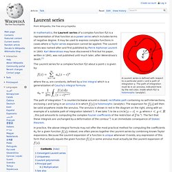
The path of integration must lie in an annulus, indicated here by the red color, inside which f(z) is holomorphic (analytic). In mathematics, the Laurent series of a complex function f(z) is a representation of that function as a power series which includes terms of negative degree. It may be used to express complex functions in cases where a Taylor series expansion cannot be applied. The Laurent series was named after and first published by Pierre Alphonse Laurent in 1843. Karl Weierstrass may have discovered it first but his paper, written in 1841, was not published until much later, after Weierstrass's death.[1]
Laplace transform. History[edit] The Laplace transform is named after mathematician and astronomer Pierre-Simon Laplace, who used a similar transform (now called z transform) in his work on probability theory.
The current widespread use of the transform came about soon after World War II although it had been used in the 19th century by Abel, Lerch, Heaviside, and Bromwich. From 1744, Leonhard Euler investigated integrals of the form as solutions of differential equations but did not pursue the matter very far.[2] Joseph Louis Lagrange was an admirer of Euler and, in his work on integrating probability density functions, investigated expressions of the form which some modern historians have interpreted within modern Laplace transform theory.[3][4][clarification needed] akin to a Mellin transform, to transform the whole of a difference equation, in order to look for solutions of the transformed equation. Formal power series. Introduction[edit] A formal power series can be loosely thought of as an object that is like a polynomial, but with infinitely many terms.
Alternatively, for those familiar with power series (or Taylor series), one may think of a formal power series as a power series in which we ignore questions of convergence by not assuming that the variable X denotes any numerical value (not even an unknown value). For example, consider the series If we studied this as a power series, its properties would include, for example, that its radius of convergence is 1. However, as a formal power series, we may ignore this completely; all that is relevant is the sequence of coefficients [1, −3, 5, −7, 9, −11, ...]. Finite impulse response. The impulse response (that is, the output in response to a Kronecker delta input) of an Nth-order discrete-time FIR filter lasts exactly N + 1 samples (from first nonzero element through last nonzero element) before it then settles to zero.
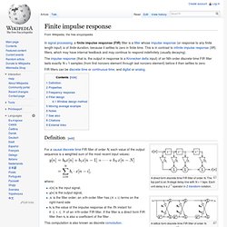
FIR filters can be discrete-time or continuous-time, and digital or analog. Convolution. Computing the inverse of the convolution operation is known as deconvolution.
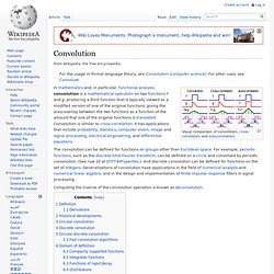
Definition[edit] The convolution of f and g is written f∗g, using an asterisk or star. Recurrence relation. The term difference equation sometimes (and for the purposes of this article) refers to a specific type of recurrence relation.
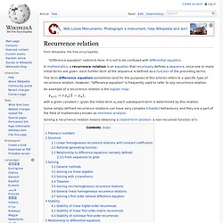
However, "difference equation" is frequently used to refer to any recurrence relation. An example of a recurrence relation is the logistic map: with a given constant r; given the initial term x0 each subsequent term is determined by this relation. Some simply defined recurrence relations can have very complex (chaotic) behaviours, and they are a part of the field of mathematics known as nonlinear analysis. Solving a recurrence relation means obtaining a closed-form solution: a non-recursive function of n. Fibonacci numbers[edit] The Fibonacci numbers are the archetype of a linear, homogeneous recurrence relation with constant coefficients (see below).
With seed values: Explicitly, recurrence yields the equations: etc. Z-transform. In mathematics and signal processing, the Z-transform converts a discrete-time signal, which is a sequence of real or complex numbers, into a complex frequency domain representation.
It can be considered as a discrete-time equivalent of the Laplace transform. This similarity is explored in the theory of time scale calculus. History[edit] The basic idea now known as the Z-transform was known to Laplace, and re-introduced in 1947 by W. Hurewicz as a tractable way to solve linear, constant-coefficient difference equations.[1] It was later dubbed "the z-transform" by Ragazzini and Zadeh in the sampled-data control group at Columbia University in 1952.[2][3] The modified or advanced Z-transform was later developed and popularized by E.