
Statistical classification. In machine learning and statistics, classification is the problem of identifying to which of a set of categories (sub-populations) a new observation belongs, on the basis of a training set of data containing observations (or instances) whose category membership is known.
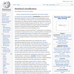
An example would be assigning a given email into "spam" or "non-spam" classes or assigning a diagnosis to a given patient as described by observed characteristics of the patient (gender, blood pressure, presence or absence of certain symptoms, etc.). In the terminology of machine learning,[1] classification is considered an instance of supervised learning, i.e. learning where a training set of correctly identified observations is available.
The corresponding unsupervised procedure is known as clustering, and involves grouping data into categories based on some measure of inherent similarity or distance. Terminology across fields is quite varied. Relation to other problems[edit] Linear classifier. Definition[edit] In this case, the solid and empty dots can be correctly classified by any number of linear classifiers.
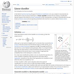
H1 (blue) classifies them correctly, as does H2 (red). H2 could be considered "better" in the sense that it is also furthest from both groups. H3 (green) fails to correctly classify the dots. If the input feature vector to the classifier is a real vector , then the output score is. Hierarchical classifier. Application[edit] There are a lot of similar applications that can also be tackled by hierarchical classification such as written text recognition[clarification needed - ambiguous term], robot awareness, etc.

It is possible that mathematical models and problem solving methods can also be represented in this fashion. [citation needed] If this is the case, future research in this area could lead to very successful automated theorem provers across multiple domain. Such developments would be very powerful,[according to whom?] But is yet unclear how exactly these models are applicable. Similar models[edit] Neuroscience's perspective on the workings of the human cortex also serves as a similar model. ROC curves and classification. To get back to a question asked after the last course (still on non-life insurance), I will spend some time to discuss ROC curve construction, and interpretation.

Consider the dataset we’ve been using last week, > db = read.table(" > attach(db) The first step is to get a model. For instance, a logistic regression, where some factors were merged together, > X3bis=rep(NA,length(X3)) > X3bis[X3%in%c("A","C","D")]="ACD" > X3bis[X3%in%c("B","E")]="BE" > db$X3bis=as.factor(X3bis) > reg=glm(Y~X1+X2+X3bis,family=binomial,data=db) From this model, we can predict a probability, not a variable, > S=predict(reg,type="response") Let denote this variable (actually, we can use the score, or the predicted probability, it will not change the construction of our ROC curve).
Variable. . , so that. Assessing the precision of classification tree model predictions. My last post focused on the use of the ctree procedure in the R package party to build classification tree models.

These models map each record in a dataset into one of M mutually exclusive groups, which are characterized by their average response. For responses coded as 0 or 1, this average may be regarded as an estimate of the probability that a record in the group exhibits a “positive response.” This interpretation leads to the idea discussed here, which is to replace this estimate with the size-corrected probability estimate I discussed in my previous post (Screening for predictive characteristics). Also, as discussed in that post, these estimates provide the basis for confidence intervals that quantify their precision, particularly for small groups.
The above plot provides a simple illustration of the results that can be obtained using the addz2ci procedure, in a case where some groups are small enough for these size-corrections to matter. Classification Tree Models. Orthogonal Partial Least Squares (OPLS) in R. I often need to analyze and model very wide data (variables >>>samples), and because of this I gravitate to robust yet relatively simple methods.

In my opinion partial least squares (PLS) is a particular useful algorithm. Simply put, PLS is an extension of principal components analysis (PCA), a non-supervised method to maximizing variance explained in X, which instead maximizes the covariance between X and Y(s). Orthogonal partial least squares (OPLS) is a variant of PLS which uses orthogonal signal correction to maximize the explained covariance between X and Y on the first latent variable, and components >1 capture variance in X which is orthogonal (or unrelated) to Y. Because R does not have a simple interface for OPLS, I am in the process of writing a package, which depends on the existing package pls. Today I wanted to make a small example of conducting OPLS in R, and at the same time take a moment to try out the R package knitr and RStudio for markdown generation.
Classification with O-PLS-DA. Partial least squares (PLS) is a versatile algorithm which can be used to predict either continuous or discrete/categorical variables.

Classification with PLS is termed PLS-DA, where the DA stands for discriminant analysis. The PLS-DA algorithm has many favorable properties for dealing with multivariate data; one of the most important of which is how variable collinearity is dealt with, and the model’s ability to rank variables’ predictive capacities within a multivariate context. Classification with O-PLS-DA.