
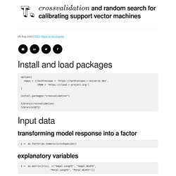
`crossvalidation` and random search for calibrating support vector machines. Options( repos = c(techtonique = ' CRAN = ' install.packages("crossvalidation") library(crossvalidation)library(e1071) transforming model response into a factor y <- as.factor(as.numeric(iris$Species)) explanatory variables X <- as.matrix(iris[, c("Sepal.Length", "Sepal.Width", "Petal.Length", "Petal.Width")]) There are many, many ways to maximize this objective function. simulation of SVM’s hyperparameters’ matrix.
Naive Bayes Classification in R » Prediction Model » finnstats. Naive Bayes Classification in R, In this tutorial, we are going to discuss the prediction model based on Naive Bayes classification.
Naive Bayes is a classification technique based on Bayes’ Theorem with an assumption of independence among predictors. The Naive Bayes model is easy to build and particularly useful for very large data sets. When you have a large dataset think about Naive classification. Deep Neural Network in R » Keras & Tensor Flow finnstats.
Neural Network in R, Neural Network is just like a human nervous system, which is made up of interconnected neurons, in other words, a neural network is made up of interconnected information processing units.
The neural network draws from the parallel processing of information, which is the strength of this method. A neural network helps us to extract meaningful information and detect hidden patterns from complex data sets. A neural network is considered one of the most powerful techniques in the data science world. Machine Learning with R: A Complete Guide to Decision Trees - Appsilon. Decision Trees with R Decision trees are among the most fundamental algorithms in supervised machine learning, used to handle both regression and classification tasks.

In a nutshell, you can think of it as a glorified collection of if-else statements, but more on that later. Support Vector Regression Tutorial for Machine Learning - Analytics Vidhya. Unlocking a New World with the Support Vector Regression Algorithm Support Vector Machines (SVM) are popularly and widely used for classification problems in machine learning.

Julia Silge - Tuning random forest hyperparameters with #TidyTuesday trees data. I’ve been publishing screencasts demonstrating how to use the tidymodels framework, from first steps in modeling to how to tune more complex models.

Today, I’m using a #TidyTuesday dataset from earlier this year on trees around San Francisco to show how to tune the hyperparameters of a random forest model and then use the final best model. Here is the code I used in the video, for those who prefer reading instead of or in addition to video. Explore the data Our modeling goal here is to predict the legal status of the trees in San Francisco in the #TidyTuesday dataset. This isn’t this week’s dataset, but it’s one I have been wanting to return to. Let’s build a model to predict which trees are maintained by the San Francisco Department of Public Works and which are not. Moodle. The Support Vector Machine algorithm is effective for balanced classification, although it does not perform well on imbalanced datasets.
The SVM algorithm finds a hyperplane decision boundary that best splits the examples into two classes. The split is made soft through the use of a margin that allows some points to be misclassified. By default, this margin favors the majority class on imbalanced datasets, although it can be updated to take the importance of each class into account and dramatically improve the performance of the algorithm on datasets with skewed class distributions. This modification of SVM that weighs the margin proportional to the class importance is often referred to as weighted SVM, or cost-sensitive SVM.
In this tutorial, you will discover weighted support vector machines for imbalanced classification. After completing this tutorial, you will know: Let’s get started. Auditor: a guided tour through residuals. Machine learning is a hot topic nowadays, thus there is no need to convince anyone about its usefulness.

ML models are being successfully applied in biology, medicine, finance, and so on. Thanks to modern software, it is easy to train even a complex model that fits the training data and results in high accuracy on the test set. The problem arises when poorly verified model fails confronted with real-world data.
In this post, we would like to describe auditor package for visual auditing of residuals of machine learning models. A residual is the difference between the observed value and the value predicted by a model. Does the model fit the data? Before we start our journey with the auditor, let us focus on linear models. However, this function can generate plots only for linear models and some of these plots are not extendable to other models.
TensorFlow for R: So, how come we can use TensorFlow from R? Which computer language is most closely associated with TensorFlow?

While on the TensorFlow for R blog, we would of course like the answer to be R, chances are it is Python (though TensorFlow has official bindings for C++, Swift, Javascript, Java, and Go as well). So why is it you can define a Keras model as library(keras) model <- keras_model_sequential() %>% layer_dense(units = 32, activation = "relu") %>% layer_dense(units = 1) (nice with %>%s and all!) – then train and evaluate it, get predictions and plot them, all that without ever leaving R? The short answer is, you have keras, tensorflow and reticulate installed. reticulate embeds a Python session within the R process. This post first elaborates a bit on the short answer. Introducing mlrPlayground.
First of all You may ask yourself how is this name ‘mlrPlayground’ even justified?

What a person dares to put two such opposite terms in a single word and expects people to take him seriously? I assume most of you know ‘mlr’, for those who don’t: It is a framework offering a huge variety of tools for simplifying machine learning tasks in R. Quite the opposite from a place, where you can play with your best friends, make new friends, live out your fantasies and just have a great time the whole day until your parents pick you up. Well, for most of the readers here this may not be the case anymore – we know, we are still young in our heart, but let’s be honest … For sure, we all have those memories and definitely have certain associations with the word ‘Playground’. The idea The idea behind this project was to offer a platform in the form of a Shiny web application, in which a user can try out different kinds of learners provided by the mlr package. Patrick Schratz. The mlr-org team is very proud to present the initial release of the mlr3 machine-learning framework for R. mlr3 comes with a clean object-oriented-design using the R6 class system.
With this, it overcomes the limitations of R’s S3 classes. A Gentle Introduction to tidymodels. By Edgar Ruiz Recently, I had the opportunity to showcase tidymodels in workshops and talks. Because of my vantage point as a user, I figured it would be valuable to share what I have learned so far. Let’s begin by framing where tidymodels fits in our analysis projects. The diagram above is based on the R for Data Science book, by Wickham and Grolemund. The version in this article illustrates what step each package covers. It is important to clarify that the group of packages that make up tidymodels do not implement statistical models themselves. In a way, the Model step itself has sub-steps. iBreakDown plots for Sinking of the RMS Titanic. DALEX for keras and parsnip – SmarterPoland.pl. DALEX is a set of tools for explanation, exploration and debugging of predictive models.
The nice thing about it is that it can be easily connected to different model factories. Recently Michal Maj wrote a nice vignette how to use DALEX with models created in keras (an open-source neural-network library in python with an R interface created by RStudio). Find the vignette here.
Shapper is on CRAN, it’s an R wrapper over SHAP explainer for black-box models – SmarterPoland.pl. Written by: Alicja Gosiewska In applied machine learning, there are opinions that we need to choose between interpretability and accuracy. However in field of the Interpretable Machine Learning, there are more and more new ideas for explaining black-box models.
One of the best known method for local explanations is SHapley Additive exPlanations (SHAP). The SHAP method is used to calculate influences of variables on the particular observation. This method is based on Shapley values, a technique borrowed from the game theory. The R package shapper is a port of the Python library shap.
A tutorial on tidy cross-validation with R - Econometrics and Free Software. Set up Let’s load the needed packages: library("tidyverse") library("tidymodels") library("parsnip") library("brotools") library("mlbench") Load the data, included in the {mlrbench} package: data("BostonHousing2") I will train a random forest to predict the housing price, which is the cmedv column: The tidy caret interface in R – poissonisfish.
Visualize the Business Value of your Predictive Models with modelplotr. ModelDown: a website generator for your predictive models – SmarterPoland.pl. I love the pkgdown package.
How to implement Random Forests in R – R-posts.com. Imagine you were to buy a car, would you just go to a store and buy the first one that you see? No, right? You usually consult few people around you, take their opinion, add your research to it and then go for the final decision. GitHub - mljar/mljar-api-R: R wrapper for MLJAR API. The one function call you need to know as a data scientist: h2o.automl. Introduction. Radial kernel Support Vector Classifier. Random Forests in R. Standardisation.
Easy Cross Validation in R with `modelr` · I'm Jacob. Ensembles Of ML Algos. Observation and Performance Window - Listen Data. The first step of building a predictive model is to define a target variable. For that we need to define the observation and performance window. Observation Window It is the period from where independent variables /predictors come from. In other words, the independent variables are created considering this period (window) only. Practicing Machine Learning Techniques in R with MLR Package. Using caret to compare models.
Cross-Validation for Predictive Analytics Using R - MilanoR. Implementation of 19 Regression algorithms in R using CPU performance data. - Data Science-Zing.
Yet Another Blog in Statistical Computing. Vik's Blog - Writings on machine learning, data science, and other cool stuff. Bagging, aka bootstrap aggregation, is a relatively simple way to increase the power of a predictive statistical model by taking multiple random samples(with replacement) from your training data set, and using each of these samples to construct a separate model and separate predictions for your test set. These predictions are then averaged to create a, hopefully more accurate, final prediction value. One can quickly intuit that this technique will be more useful when the predictors are more unstable. In other words, if the random samples that you draw from your training set are very different, they will generally lead to very different sets of predictions. This greater variability will lead to a stronger final result. When the samples are extremely similar, all of the predictions derived from the samples will likewise be extremely similar, making bagging a bit superfluous.
Okay, enough theoretical framework. Confidence Intervals for Random Forests. Compare The Performance of Machine Learning Algorithms in R. Predicting wine quality using Random Forests. Kickin’ it with elastic net regression – On the lambda. Self-Organising Maps for Customer Segmentation using R. Using C4.5 to predict Diabetes in Pima Indian Women. Down-Sampling Using Random Forests — Applied Predictive Modeling.