
GAMs in R by Noam Ross. Generalized Additive Models. GAMs are simply a class of statistical Models in which the usual Linear relationship between the Response and Predictors are replaced by several Non linear smooth functions to model and capture the Non linearities in the data.These are also a flexible and smooth technique which helps us to fit Linear Models which can be either linearly or non linearly dependent on several Predictors \(X_i\) to capture Non linear relationships between Response and Predictors.In this article I am going to discuss the implementation of GAMs in R using the 'gam' package.Simply saying GAMs are just a Generalized version of Linear Models in which the Predictors \(X_i\) depend Linearly or Non linearly on some Smooth Non Linear functions like Splines , Polynomials or Step functions etc.
The Regression Equation becomes: $$f(x) \ = y_i \ = \alpha \ + f_1(x_{i1}) \ + f_2(x_{i2}) \ + …. f_p(x_{ip}) \ + \epsilon_i$$ where the functions \(f_1,f_2,f_3,….f_p \) are different Non Linear Functions on variables \(X_p\) . Generalized Additive Models (GAM) The methods available in Generalized Additive Models are implementations of techniques developed and popularized by Hastie and Tibshirani (1990).
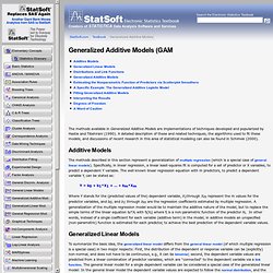
A detailed description of these and related techniques, the algorithms used to fit these models, and discussions of recent research in this area of statistical modeling can also be found in Schimek (2000). Additive Models The methods described in this section represent a generalization of multiple regression (which is a special case of general linear models). Specifically, in linear regression, a linear least-squares fit is computed for a set of predictor or X variables, to predict a dependent Y variable. The well known linear regression equation with m predictors, to predict a dependent variable Y, can be stated as: Y = b0 + b1*X1 + ... + bm*Xm.
Generalized Additive Models in R. Generalized additive models in R GAMs in R are a nonparametric extension of GLMs, used often for the case when you have no a priori reason for choosing a particular response function (such as linear, quadratic, etc.) and want the data to 'speak for themselves'.
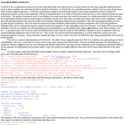
GAMs do this via a smoothing function, similar to what you may already know about locally weighted regressions. GAMs take each predictor variable in the model and separate it into sections (delimited by 'knots'), and then fit polynomial functions to each section separately, with the constraint that there are no kinks at the knots (second derivatives of the separate functions are equal at the knots). The number of parameters used for such fitting is obviously more than what would be necessary for a simpler parametric fit to the same data, but computational shortcuts mean the model degrees of freedom is usually lower than what you might expect from a line with so much 'wiggliness'.
Ls1 = loess(cover>0~elev,data=dat5) Animating smoothing uncertainty in a GAM. Gam plots. Glm and gam confidence intervals. Website Performance Monitoring > How can I obtain the values of confidence intervals from gam anf glm > objects?

- Vp in the gam object is the covariance matrix of the posterior distribution of the gam parameters under a certian Bayesian model of smoothing, the mean of this distribution is the parameter estimates (coefficients). In the large sample limit the distribution is normal (exactly so for normal errors and identity link). - predict.gam() can give standard errors for any prediction that you ask it to make (on the scale of the linear predictor these are exact and do not, for example, rely on any approximations like the estimators of the smooths being independent).
CI's then obtainable from the large sample normal result. Regression with Splines: Should we care about Non-Significant Components? Following the course of this morning, I got a very interesting question from a student of mine.

The question was about having non-significant components in a splineregression. Should we consider a model with a small number of knots and all components significant, or one with a (much) larger number of knots, and a lot of knots non-significant? My initial intuition was to prefer the second alternative, like in autoregressive models in R. When we fit an AR(6) model, it’s not really a big deal if most coefficients are not significant (but the last one). It’s won’t affect much the forecast. Visualisations for GAMs. The mgcViz R package offers visual tools for Generalized Additive Models (GAMs).
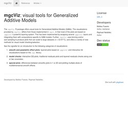
The visualizations provided by mgcViz differs from those implemented in mgcv, in that most of the plots are based on ggplot2’s powerful layering system. This has been implemented by wrapping several ggplot2 layers and integrating them with computations specific to GAM models. Further, mgcViz uses binning and/or sub-sampling to produce plots that can scale to large datasets (n = O(10^7)), and offers a variety of new methods for visual model checking/selection.
See the vignette for an introduction to the following categories of visualizations: smooth and parametric effect plots: layered plots based on ggplot2 and interactive 3d visualizations based on the rgl library;model checks: interactive QQ-plots, traditional residuals plots and layered residuals checks along one or two covariates;special plots: differences-between-smooths plots in 1 or 2D and plotting multiple slices of multidimensional smooth effects. Introducing gratia. I use generalized additive models (GAMs) in my research work.
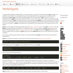
I use them a lot! Simon Wood’s mgcv package is an excellent set of software for specifying, fitting, and visualizing GAMs for very large data sets. Despite recently dabbling with brms, mgcv is still my go-to GAM package. The only down-side to mgcv is that it is not very tidy-aware and the ggplot-verse may as well not exist as far as it is concerned. This in itself is no bad thing, though as someone who uses mgcv a lot but also prefers to do my plotting with ggplot2, this lack of awareness was starting to hurt. Gratia is an R package for working with GAMs fitted with gam(), bam() or gamm() from mgcv or gamm4() from the gamm4 package, although functionality for handling the latter is not yet implement. gratia provides functions to replace the base-graphics-based plot.gam() and gam.check() that mgcv provides with ggplot2-based versions.
Extrapolating with B splines and GAMs. An issue that often crops up when modelling with generlaized additive models (GAMs), especially with time series or spatial data, is how to extrapolate beyond the range of the data used to train the model?
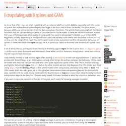
The issue arises because GAMs use splines to learn from the data using basis functions.