
FindFn (sos package) FindFn(string, maxPages = 20) Do a search for functions, which opens an interactive HTML page of results.
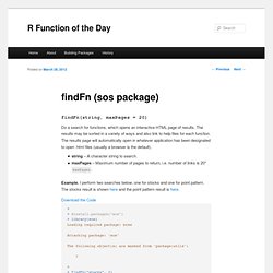
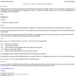
The results may be sorted in a variety of ways and also link to help files for each function. The results page will automatically open in whatever application has been designated to open .html files (usually a browser is the default). string – A character string to search.maxPages – Maximum number of pages to return, i.e. number of links is 20*maxPages. Example. Find hidden code for functions. Retrieve an R Object, Including from a Namespace. Description These functions locate all objects with name matching their argument, whether visible on the search path, registered as an S3 method or in a namespace but not exported. getAnywhere() returns the objects and argsAnywhere() returns the arguments of any objects that are functions.
Usage. Finding the code for a ‘hidden’ function in R. Finding the code for a ‘hidden’ function in R If you want to understand what a certain function is doing, or you want to adapt it, you can type in the function without bracket on the command line.
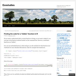
However, sometimes functions are ‘hidden’. Get. Magic empty bracket. Print_fs: Print File Structure. We at STATWORX work a lot with R and we often use the same little helper functions within our projects.

These functions ease our daily work life by reducing repetitive code parts or by creating overviews of our projects. At first, there was no plan to make a package, but soon I realised, that it will be much easier to share and improve those functions, if they are within a package. Up till the 24th December I will present one function each day from helfRlein. So, on the 14th day of Christmas my true love gave to me… What can it do?
This little helper returns the folder structure of a given path. Symmetric set differences in R. My .Rprofile contains a collection of convenience functions and function abbreviations.
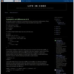
These are either functions I use dozens of times a day and prefer not to type in full: ## my abbreviation of head() h <- function(x, n=10) head(x, n) ## and summary() ss <- summary Or problems that I'd rather figure out once, and only once: ## example: ## between( 1:10, 5.5, 6.5 ) between <- function(x, low, high, ineq=F) { ## like SQL between, return logical index if (ineq) { x >= low & x <= high } else { x > low & x < high } } One of these "problems" that's been rattling around in my head is the fact that setdiff(x, y) is asymmetric, and has no options to modify this. Boolean operators && and. Key R Operators. Only recently have I discovered the true power of some the operators in R.

Here are some tips on some underused operators in R: The %in% operator This funny looking operator is very handy. It’s short for testing if several values appear in an object. For instance. Skimr for useful and tidy summary statistics. Like every R user who uses summary statistics (so, everyone), our team has to rely on some combination of summary functions beyond summary() and str().
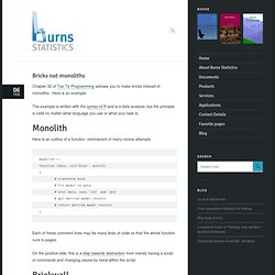
But we found them all lacking in some way because they can be generic, they don't always provide easy-to-operate-on data structures, and they are not pipeable. What we wanted was a frictionless approach for quickly skimming useful and tidy summary statistics as part of a pipeline. And so at rOpenSci #unconf17, we developed skimr. In a nutshell, skimr will create a skim_df object that can be further operated upon or that provides a human-readable printout in the console. It presents reasonable default summary statistics for numerics, factors, etc, and lists counts, and missing and unique values. Backstory. Bricks not monoliths. Chapter 32 of Tao Te Programming advises you to make bricks instead of monoliths.
3 dots construct in R. There is a mechanism that allows variability in the arguments given to R functions.
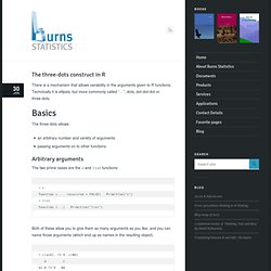
Technically it is ellipsis, but more commonly called “…”, dots, dot-dot-dot or three-dots. Basics The three-dots allows: an arbitrary number and variety of argumentspassing arguments on to other functions Arbitrary arguments. Ellipsis. Lexical scope and function closures in R. Introduction R is different to many “easy to use” statistical software packages – it expects to be given commands at the R command prompt.
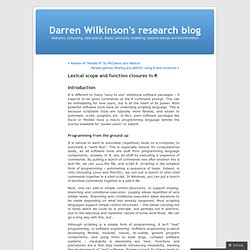
This can be intimidating for new users, but is at the heart of its power. Most powerful software tools have an underlying scripting language. This is because scriptable tools are typically more flexible, and easier to automate, script, program, etc. In fact, even software packages like Excel or Minitab have a macro programming language behind the scenes available for “power users” to exploit. Programming from the ground up. Tidysearch. Geocoding function. This is a very simple function to perform geocoding using the Google Maps API: Essentially, users need to get an API key from google and then use as an input (string) for the function. The function itself is very simple, and it is an adaptation of some code I found on-line (unfortunately I did not write down where I found the original version so I do not have a way to reference the source, sorry!!). GeoCodes <- getGeoCode(gcStr="11 via del piano, empoli", key) To use the function we simply need to include an address, and it will return its coordinates in WGS84.
Checkdir. We at STATWORX work a lot with R and we often use the same little helper functions within our projects. These functions ease our daily work life by reducing repetitive code parts or by creating overviews of our projects. At first, there was no plan to make a package, but soon I realised, that it will be much easier to share and improve those functions, if they are within a package. Up till the 24th December I will present one function each day from helfRlein. So, on the 1st day of Christmas my true love gave to me… Don't forget the "utils" package in R.
With thousands of powerful packages, it’s easy to glaze over the libraries that come preinstalled with R. Thus, this post will talk about some of the cool functions in the utils package, which comes with a standard installation of R. While utils comes with several familiar functions, like read.csv, write.csv, and help, it also contains over 200 other functions. readClipboard and writeClipboard One of my favorite duo of functions from utils is readCLipboard and writeClipboard. Helpers for 'OOP' in R. Primitive Functions List.
Practicing static typing in R: Prime directive on trusting our functions with object oriented programming. The creator of S language which R is derived from John Chambers said in one of his books Software for data analysis programming with R: ...This places an obligation on all creators of software to program in such away that the computations can be understood and trusted. This obligationI label the Prime Directive. He was referring to prime directive from Star Trek. Debugging with RStudio. Introduction. Debugging in R: How to Easily and Efficiently Conquer Errors in Your Code. General suggestions for debugging R. How to write and debug an R function. Data and Code Download. Tracking down errors in R. It's that moment we all know and love, somewhere in our code something has gone wrong. We think we have done everything right, but instead of expected glory we find only terse red text lain below our lintel.
Catching errors in R and trying something else. Translating Weird R Errors. Easy data validation with the validate package. The validate package is our attempt to make checking data against domain knowledge as easy as possible. R: Bug Reporting in R. Debugging techniques in RStudio. 4 ways to not just read the code, but delve into it step-by-step. As pointed out by a recent read the R source post on the R hub’s website, reading the actual code, not just the documentation is a great way to learn more about programming and implementation details.
Handling R errors the rlang way. Every day we deal with errors, warnings and messages while writing, debugging or reviewing code. Example of unit testing R code with testthat. Mocking is catching. When writing unit tests for a package, you might find yourself wondering about how to best test the behaviour of your package.