
DSM R manual 2013. Keyboard Shortcuts. Spencer Guerrero - University of Illinois at Urbana-Champaign. So I decided for an R example I would just walk through a complete statistical analysis from the very first steps for some publicly available data.
The funny thing about me saying a “complete” analysis is that I don’t think any of my statistical analysis are ever “finished” in that there is always one more thing I could examine or plot or explore. I do always reach a good stopping point though after answering what I set out to investigate. So goodluck. Beside walking through getting the data cleaned up and into a “final” form for analysis.
I have just two further pages. If I was to create another page I would go over quantifying the max and min daily temperature distributions for each daily average temperature and calculate the mean and standard deviation of each distribution and compare the mean to the avg daily temperature. Introduction to raster based analysis in R. Short refcard. Headwater Analytics - Blog.
Data Types. R has a wide variety of data types including scalars, vectors (numerical, character, logical), matrices, data frames, and lists.
Vectors a <- c(1,2,5.3,6,-2,4) # numeric vector b <- c("one","two","three") # character vector c <- c(TRUE,TRUE,TRUE,FALSE,TRUE,FALSE) #logical vector Refer to elements of a vector using subscripts. a[c(2,4)] # 2nd and 4th elements of vector Matrices All columns in a matrix must have the same mode(numeric, character, etc.) and the same length. Mymatrix <- matrix(vector, nrow=r, ncol=c, byrow=FALSE, dimnames=list(char_vector_rownames, char_vector_colnames)) byrow=TRUE indicates that the matrix should be filled by rows. byrow=FALSE indicates that the matrix should be filled by columns (the default). dimnames provides optional labels for the columns and rows. # generates 5 x 4 numeric matrix y<-matrix(1:20, nrow=5,ncol=4)
15 Easy Solutions To Your Data Frame Problems In R. R's data frames regularly create somewhat of a furor on public forums like Stack Overflow and Reddit.
Starting R users often experience problems with the data frame in R and it doesn't always seem to be straightforward. But does it really need to be so? Well, not necessarily. With today's post, DataCamp wants to show you that data frames don't need to be hard: we offer you 15 easy, straightforward solutions to the most frequently occurring problems with data.frame. These issues have been selected from the most recent and sticky or upvoted Stack Overflow posts.
The Root: What's A Data Frame? VALUE TS1 D02 RIntro. RStudio - Cheatsheets. Introduction to MATLAB. Introduction To MATLAB Programming. Get Started In R: A Complete Beginners Workbook. This is a step-by-step learning guide cum practice workbook for beginners to get started with R.
It is created especially for newbies who prefer to learn the language from scratch and want to get up to speed very quickly without referring too many resources. By the end of this page you will have a pretty good understanding of the language and be in a position to take on more challenging techniques illustrated in rest of this website. I assume that you have R installed and are ready to follow along, typing the codes in to your R console as you learn. Percentile. The nth percentile of an observation variable is the value that cuts off the first n percent of the data values when it is sorted in ascending order.
Problem Find the 32nd, 57th and 98th percentiles of the eruption durations in the data set faithful. Solution We apply the quantile function to compute the percentiles of eruptions with the desired percentage ratios. > duration = faithful$eruptions # the eruption durations > quantile(duration, c(.32, .57, .98)) 32% 57% 98% 2.3952 4.1330 4.9330 Answer The 32nd, 57th and 98th percentiles of the eruption duration are 2.3952, 4.1330 and 4.9330 minutes respectively.
Exercise Find the 17th, 43rd, 67th and 85th percentiles of the eruption waiting periods in faithful. Note. Data Mining With R: TIME SERIES using R. FITTING ARIMA MODEL in RAuto Regressive Integrated Moving Average ( ARIMA) model is generalisation of Auto Regressive Moving Average Model (ARMA) and used to predict future points in Time series.But what is time series , Acc to google "A time series is a sequence of data points, typically consisting of successive measurements made over a time interval.
Examples of time series are ocean tides, counts of sunspots, and the daily closing value of the Dow Jones Industrial Average. " and more in a general way it is a series of values of a quantity obtained at successive times, often with equal intervals between them.ARIMA models are defined for stationary time series , stationary time series is one whose mean, variance, autocorrelation are all constant over time. Mann-Whitney-Wilcoxon Test. Two data samples are independent if they come from distinct populations and the samples do not affect each other.
Using the Mann-Whitney-Wilcoxon Test, we can decide whether the population distributions are identical without assuming them to follow the normal distribution. Example In the data frame column mpg of the data set mtcars, there are gas mileage data of various 1974 U.S. automobiles. > mtcars$mpg [1] 21.0 21.0 22.8 21.4 18.7 ... Meanwhile, another data column in mtcars, named am, indicates the transmission type of the automobile model (0 = automatic, 1 = manual). TimeSeriesR2004.pdf.
Learning_Module_3.pdf. Welcome to a Little Book of R for Time Series! — Time Series 0.2 documentation. Forecasting: principles and practice. Welcome to our online textbook on forecasting.
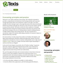
This textbook is intended to provide a comprehensive introduction to forecasting methods and to present enough information about each method for readers to be able to use them sensibly. We don’t attempt to give a thorough discussion of the theoretical details behind each method, although the references at the end of each chapter will fill in many of those details. The book is written for three audiences: (1) people finding themselves doing forecasting in business when they may not have had any formal training in the area; (2) undergraduate students studying business; (3) MBA students doing a forecasting elective. We use it ourselves for a second-year subject for students undertaking a Bachelor of Commerce degree at Monash University, Australia. For most sections, we only assume that readers are familiar with algebra, and high school mathematics should be sufficient background. Use the table of contents on the right to browse the book.
Tau. Wq-package.pdf. R Resources.
Producing Simple Graphs with R. MATLAB Central - Jeff Burkey. R for Journalists. Learn R. DataVisualization. Code School - Try R. R. Syllabus. Lectures: none (directed reading course) Textbook: Class Notes (see references below) References: Online MATLAB tutorials and references: MATLAB guides Provided with the Matlab installation.
Code School - Try R. Programming R. Short-refcard.pdf. Spi program alternative method. Spi.