
A Community Site for R – Sponsored by Revolution Analytics. Shiny - Tutorial. The How to Start Shiny video series will take you from R programmer to Shiny developer.

Watch the complete tutorial here, or jump to a specific chapter by clicking a link below. The entire tutorial is two hours and 25 minutes long. R Language. Rank tests. We learned how the sample mean and sd are susceptible to outliers.
The t-test is based on these measures and is susceptible as well. The Wilcox signed-rank test provides and alternative. In the code below we perform a t-test on data for which the null is true but we change one observation by mistakes in each sample and the values incorrectly entered are different. Robust summaries and log transformation.
The normal apporximatiion is often useful when analyzing life sciences data.
However, due to the complexity of the measurement devices it is also common to mistakenlyobserve data points generated by an undesired process. Dplyr tutorial. What is dplyr?
Dplyr is a powerful R-package to transform and summarize tabular data with rows and columns. For another explanation of dplyr see the dplyr package vignette: Introduction to dplyr Why is it useful? The package contains a set of functions (or “verbs”) that perform common data manipulation operations such as filtering for rows, selecting specific columns, re-ordering rows, adding new columns and summarizing data. Plots to avoid. This section is based on talk by Karl W.
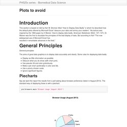
Broman titled “How to Display Data Badly” in which he described how the default plots offered by Microsoft Excel “obscure your data and annoy your readers”. His lecture was inspired by the 1984 paper by H Wainer: How to display data badly. American Statistician 38(2): 137–147}. Exploratory Data Analysis 2. We introduce EDA for univariate data.
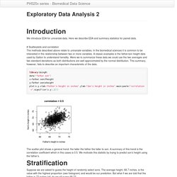
Here we describe EDA and summary statistics for paired data. # Scatterplots and correlation The methods described above relate to univariate variables. In the biomedical sciences it is common to be interested in the relationship between two or more variables. A classic examples is the father/son height data used by Galton to understand heredity. Were we to summarize these data we could use the two averages and two standard deviations as both distributions are well approximated by the normal distribution. Library(UsingR)data("father.son")x=father.son$fheighty=father.son$sheightplot(x,y,xlab="Father's height in inches",ylab="Son's height in inches",main=paste("correlation =",signif(cor(x,y),2))) The scatter plot shows a general trend: the taller the father the taller to son. Exploratory Data Analysis 1. Biases, systematic errors and unexpected variability are common in data from the life sciences.
Failure to discover these problems often leads to flawed analyses and false discoveries. As an example, consider that experiments sometimes fail and not all data processing pipelines, such as the t.test function in R, are designed to detect these. Yet, these pipelines still give you an answer. Furthermore, it may be hard or impossible to notice an error was made just from the reported results. Permutation tests. Suppose we have a situation in which none of the standard statistical tools apply.
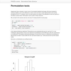
We have computed a summary statisitic, such as the difference in mean, but do not have a useful approximation such as that provided by the CLT. Monte Carlo methods. Computers can be used to generate pseudo-random numbers.
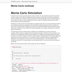
For most practicaly purposes these pseudo-random numbers can be used to immitate real random variables. This permits us to examine properties of random variables using a computer instead of theoretical or analytical derivations. One very useful aspect of this concept is that we can create simulated data to test out ideas or competing methods without actually having to perform laboratory experiments.
Simulations can also be used to check theoretical or analytical results. Also, many of the theoretical results we use in statistics are based on asymptotics: they hold when the sample size goes to infinity. The technique we used to motivate random variables and null distribution was a type of monte carlo simulation. Below is the code we used to obtain random sample and then the difference: library(downloader) ## ## Attaching package: 'downloader' ## ## The following object is masked from 'package:devtools': ## ## source_url.
Association tests. The statistical tests we have covered up to know leave out a substantial portion of life science projects.
Specifically, we are referring to data that is binary, categorical and ordinal. To give a very specific example, consider genetic data where you have two genotypes (AA/Aa or aa) for cases and controls for a given disease. The statistical question is if genotype and disease are associated. Power calculations. We have used the example of the effects of two different diets on the weight of mice. Because in this illustrative example we have access to the population we know that in fact there is a substantial (about 10%) difference between the average weights of the two populations: library(downloader)url<-" <- tempfile()download(url,destfile=filename)dat <- read.csv(filename)hfPopulation <- dat[dat$Sex=="F" & dat$Diet=="hf",3]controlPopulation <- dat[dat$Sex=="F" & dat$Diet=="chow",3]mu_hf <- mean(hfPopulation)mu_control <- mean(controlPopulation)print(mu_hf - mu_control) We have also seen that in some cases, when we take a sample and perform a t-test we don’t always get a p-value smaller than 0.05.
For example, here is a case were we take sample of 5 mice and we don’t achieve statistical significance at the 0.05 level: Confidence Intervals. We have described how to compute p-values, which are ubiquitous in the life sciences. However, we do not recommend reporting p-values as the only statistical summary of your results. The reason is simple: statistical significance does not guarantee scientific significance.
With large enough sample sizes, one might detect a statistically significance difference in weight of, say, 1 microgram. But is this an important finding? Would we say a diet results in higher weight if the increase is less than a fraction of a percent? T-tests in practice. Central Limit Theorem in practice. Let’s use our data to see how well the central limit approximates sample averages from our data. We will leverage our entire population dataset to compare the results we obtain by actually sampling from the distribtuion to what the CLT predicts. library(downloader)url <- " <- tempfile()download(url,destfile=filename)dat <- read.csv(filename)head(dat) ## Sex Diet Bodyweight ## 1 F hf 31.94 ## 2 F hf 32.48 ## 3 F hf 22.82 ## 4 F hf 19.92 ## 5 F hf 32.22 ## 6 F hf 27.50 Start by selecting only female mice since males and females have different weights.
Central Limit Theorem and t-distribution. Below we will discuss two mathematical results, the Central Limit Theorem and the t-distribution, which help us to calculate probabilities of observing events, and both are often used in science to test statistical hypotheses. They have different assumptions, but both results are similar in that through mathematical formula, we are able to calculate exact probabilities of events, if we think that certain assumptions about the data hold true.
The Central Limit Theorem (or CLT) is one of the most used mathematical results in science. It tells us that when the sample size is large the average ˉY of a random sample follows a normal distribution centered at the population average μY and with standard deviation equal to the population standard deviation σY, divided by the square root of the sample size N. Two important mathematical results you need to know are that if we subtract a constant from a random variable, the mean of the new random variable shifts by that constant.
ˉY−μσY/√N √NˉYsY. Population, Samples, and Estimates. Now that we have introduced the idea of a random variable, a null distribution, and a p-value, we are ready to describe the mathematical theory that permits us to compute p-values in practice. Introduction to random variables. Introduction This course introduces the statistical concepts necessary to understand p-values and confidence intervals. These terms are ubiquitous in the life science literature. Let’s look at this paper as an example. Note that the abstract has this statement: