
Time Series Analysis -A Beginner Friendly Guide - Analytics Vidhya. Introduction to Functional Data Analysis with R. By Joseph Rickert Suppose you have data that looks something like this.
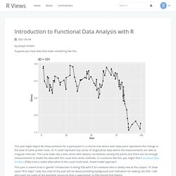
This plot might depict 80 measurements for a participant in a clinical trial where each data point represents the change in the level of some protein level. Or it could represent any series of longitudinal data where the measurements are take at irregular intervals. The curve looks like a time series with obvious correlations among the points, but there are not enough measurements to model the data with the usual time series methods. In a scenario like this, you might find Functional Data Analysis (FDA) to be a viable alternative to the usual multi-level, mixed model approach. This post is meant to be a “gentle” introduction to doing FDA with R for someone who is totally new to the subject.
FDA is a branch of statistics that deals with data that can be conceptualized as a function of an underlying, continuous variable. First Steps Note that we are placing the knots at times equally spaced over the 100 day time span. Introduction to Time Series in R. Introduction to the forecastLM package. I am pleased to announce a new R package - forecastLM.
The package, as the name implies, provides applications for forecasting regular time series data with a linear regression model (based on the lm function from the stats package). It supports both ts and tsibble objects as inputs and enables simple extractions of features from the input object on the fly. Example for such features: Single or Multiple seasonal components (when applicable)Different types of trends (regular, log, exponential, polynomial)Adding past lagsPiecewise regressionVariables selection with stepwise regressionHandle events and outliers In addition, it provides interactive data visualization tools utilizing the plotly package. Installation. Bootstrapping time series for improving forecasting accuracy – Peter Laurinec – Time series data mining in R. Bratislava, Slovakia.
Bootstrapping time series?
It is meant in a way that we generate multiple new training data for statistical forecasting methods like ARIMA or triple exponential smoothing (Holt-Winters method etc.) to improve forecasting accuracy. It is called bootstrapping, and after applying the forecasting method on each new time series, forecasts are then aggregated by average or median - then it is bagging - bootstrap aggregating. It is proofed by multiple methods, e.g. in regression, that bagging helps improve predictive accuracy - in methods like classical bagging, random forests, gradient boosting methods and so on.
Introducing feasts. Feast your eyes on the latest CRAN release to the collection of tidy time series R packages.

The feasts package is feature-packed with functions for understanding the behaviour of time series through visualisation, decomposition and feature extraction. The package name feasts is an acronym summarising its key features: Feature Extraction And Statistics for Time Series. Much like Earo Wang’s tsibble package, the feasts package is designed to work with multiple series observed at any time interval. If you’ve used graphics from Rob Hyndman’s forecast package or features from tsfeatures, this package allows these features to be used seamlessly with tsibble and the tidyverse. With the package now available on CRAN, it is now easier than ever to install: install.packages("feasts")
Time series graphics using feasts. This is the second post on the new tidyverts packages for tidy time series analysis.
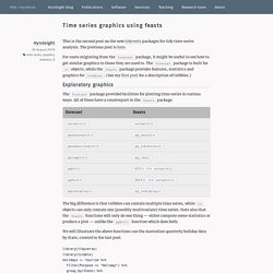
The previous post is here. For users migrating from the forecast package, it might be useful to see how to get similar graphics to those they are used to. The forecast package is built for ts objects, while the feasts package provides features, statistics and graphics for tsibbles. (See my first post for a description of tsibbles.) Exploratory graphics. Time series graphics using feasts. Tsbox 0.2: supporting additional time series classes.
The tsbox package makes life with time series in R easier.

It is built around a set of functions that convert time series of different classes to each other. They are frequency-agnostic, and allow the user to combine time series of multiple non-standard and irregular frequencies. A detailed overview of the package functionality is given in the documentation page (or in a previous blog-post). Version 0.2 is now on CRAN and provides a larger number of bugfixes. Non-standard column names are now handled correctly, and non-standard column orders are treated consistently. Forecasting: Principles and Practice. Forecast v8.3 now on CRAN. Introduction for the TSstudio Package. Seasonality analysis The TSstudio provides a variety of tools for seasonality analysis, currently supporting only monthly or quarterly data.
The monthly consumption of natural gas in the US (USgas dataset) is a good example of a seasonal pattern within time series data: # Load the US monthly natural gas consumptiondata("USgas") class(USgas) ## [1] "ts" ts_plot(USgas, title = "US Natural Gas Consumption", Xtitle = "Year", Ytitle = "Billion Cubic Feet" ) The ts_seasonal function The ts_seasonal function provides 3 types of seasonal plots: “normal” - break of a series by year, this allows identifying a seasonal pattern within the year ts_seasonal(USgas, type = "normal") “cycle” - break of a series by the cycle units (i.e. months or quarters), it can be used to identify trends and patterns between the cycle units: TSrepr - Time Series Representations in R – Peter Laurinec – Time series data mining in R. Bratislava, Slovakia. I’m happy to announce a new package that has recently appeared on CRAN, called “TSrepr” (version 1.0.0: The TSrepr package contains methods of time series representations (dimensionality reduction, feature extraction or preprocessing) and several other useful helper methods and functions.
Time series representation can be defined as follows: Let \( x \) be a time series of length \( n \), then representation of \( x \) is a model \( \hat{x} \) with reduced dimensionality \( p \) \( (p < n) \) such that \( \hat{x} \) approximates closely \( x \) (Esling and Agon (2012)). Time series representations are used for: significant reduction of the time series dimensionality emphasis on fundamental (essential) shape characteristics implicit noise handling reducing the dimension will reduce memory requirements and computational complexity of consequent machine learning methods.
Therefore, they are awesome! Time Series Forecasting with Recurrent Neural Networks. In this section, we’ll review three advanced techniques for improving the performance and generalization power of recurrent neural networks.
By the end of the section, you’ll know most of what there is to know about using recurrent networks with Keras. We’ll demonstrate all three concepts on a temperature-forecasting problem, where you have access to a time series of data points coming from sensors installed on the roof of a building, such as temperature, air pressure, and humidity, which you use to predict what the temperature will be 24 hours after the last data point. This is a fairly challenging problem that exemplifies many common difficulties encountered when working with time series.
We’ll cover the following techniques: A temperature-forecasting problem Until now, the only sequence data we’ve covered has been text data, such as the IMDB dataset and the Reuters dataset. Demo Week: Tidy Time Series Analysis with tibbletime. We’re into the fourth day of Business Science Demo Week.

We have a really cool one in store today: tibbletime, which uses a new tbl_time class that is time-aware!! For those that may have missed it, every day this week we are demo-ing an R package: tidyquant (Monday), timetk (Tuesday), sweep (Wednesday), tibbletime (Thursday) and h2o (Friday)! That’s five packages in five days! We’ll give you intel on what you need to know about these packages to go from zero to hero. Let’s take tibbletime for a spin! Previous Demo Week Demos. Tibbletime-0-0-2. Today we are introducing tibbletime v0.0.2, and we’ve got a ton of new features in store for you.
We have functions for converting to flexible time periods with the ~period formula~ and making/calculating custom rolling functions with rollify() (plus a bunch more new functionality!). We’ll take the new functionality for a spin with some weather data (from the weatherData package). However, the new tools make tibbletime useful in a number of broad applications such as forecasting, financial analysis, business analysis and more! We truly view tibbletime as the next phase of time series analysis in the tidyverse. If you like what we do, please connect with us on social media to stay up on the latest Business Science news, events and information!
Using regression trees for forecasting double-seasonal time series with trend in R – Peter Laurinec – Time series data mining in R. Bratislava, Slovakia. After blogging break caused by writing research papers, I managed to secure time to write something new about time series forecasting. This time I want to share with you my experiences with seasonal-trend time series forecasting using simple regression trees.
Classification and regression tree (or decision tree) is broadly used machine learning method for modeling. They are favorite because of these factors: simple to understand (white box) from a tree we can extract interpretable results and make simple decisions they are helpful for exploratory analysis as binary structure of tree is simple to visualize very good prediction accuracy performance very fast they can be simply tuned by ensemble learning techniques. Tidy Time Series Analysis, Part 3: The Rolling Correlation.
In the third part in a series on Tidy Time Series Analysis, we’ll use the runCor function from TTR to investigate rolling (dynamic) correlations. We’ll again use tidyquant to investigate CRAN downloads. This time we’ll also get some help from the corrr package to investigate correlations over specific timespans, and the cowplot package for multi-plot visualizations. We’ll end by reviewing the changes in rolling correlations to show how to detect events and shifts in trend. If you like what you read, please follow us on social media to stay up on the latest Business Science news, events and information! As always, we are interested in both expanding our network of data scientists and seeking new clients interested in applying data science to business and finance.
If you haven’t checked out the previous two tidy time series posts, you may want to review them to get up to speed. We’ll need to load four libraries today. Data Science for Business - Time Series Forecasting Part 3: Forecasting with Facebook's Prophet. In my last two posts (Part 1 and Part 2), I explored time series forecasting with the timekit package. In this post, I want to compare how Facebook’s prophet performs on the same dataset. Predicting future events/sales/etc. isn’t trivial for a number of reasons and different algorithms use different approaches to handle these problems.
Time series data does not behave like a regular numeric vector, because months don’t have the same number of days, weekends and holidays differ between years, etc. Because of this, we often have to deal with multiple layers of seasonality (i.e. weekly, monthly, yearly, irregular holidays, etc.). A Gentle Introduction to Autocorrelation and Partial Autocorrelation. R packages for forecast combinations. It has been well-known since at least 1969, when Bates and Granger wrote their famous paper on “The Combination of Forecasts”, that combining forecasts often leads to better forecast accuracy.
So it is helpful to have a couple of new R packages which do just that: opera and forecastHybrid. opera Opera stands for “Online Prediction by ExpeRt Aggregation”. It was written by Pierre Gaillard and Yannig Goude, and Pierre provides a nice introduction in the vignette. The thief package for R: Temporal HIErarchical Forecasting. I have a new R package available to do temporal hierarchical forecasting, based on my paper with George Athanasopoulos, Nikolaos Kourentzes and Fotios Petropoulos. (Guess the odd guy out there!) It is called “thief” – an acronym for Temporal HIErarchical Forecasting. The idea is to take a seasonal time series, and compute all possible temporal aggregations that result in an integer number of observations per year.
PSF : R Package for Pattern Sequence based Forecasting Algorithm. Introduction The Algorithm Pattern Sequence based Forecasting (PSF) was first proposed by Martinez Alvarez, et al., 2008 and then modified and suggested improvement by Martinez Alvarez, et al., 2011. The technical detailes are mentioned in referenced articles. Better prediction intervals for time series forecasts.
Forecast Combination I’ve referred several times to this blog post by Rob Hyndman in which he shows that a simple averaging of the ets() and auto.arima() functions in his {forecast} R package not only out performs ets() and auto.arima() individually (in the long run, not every time), they outperform nearly every method that was entered in the M3 competition in the year 2000. Using R for Time Series Analysis — Time Series 0.2 documentation. Introducing practical and robust anomaly detection in a time series. Both last year and this year, we saw a spike in the number of photos uploaded to Twitter on Christmas Eve, Christmas and New Year’s Eve (in other words, an anomaly occurred in the corresponding time series). Time series outlier detection (a simple R function) Teaching page: Ruey S. Tsay. R Video tutorial for Spatial Statistics: Introductory Time-Series analysis of US Environmental Protection Agency (EPA) pollution data. Download EPA air pollution data The US Environmental Protection Agency (EPA) provides tons of free data about air pollution and other weather measurements through their website.
An overview of their offer is available here: The data are provided in hourly, daily and annual averages for the following parameters: Ozone, SO2, CO,NO2, Pm 2.5 FRM/FEM Mass, Pm2.5 non FRM/FEM Mass, PM10, Wind, Temperature, Barometric Pressure, RH and Dewpoint, HAPs (Hazardous Air Pollutants), VOCs (Volatile Organic Compounds) and Lead. All the files are accessible from this page: The web links to download the zip files are very similar to each other, they have an initial starting URL: and then the name of the file has the following format: type_property_year.zip The type can be: hourly, daily or annual.
The properties are sometimes written as text and sometimes using a numeric ID. Basics of Time Series - Stationary series and Random walk. Journal of Statistical Software — Show. Time Series Analysis. CasualImpact - Determining Impact of Marketing Interventions. What is volatility? An online textbook by Rob J Hyndman and George Athanasopoulos.