
Importance of exports and economic growth, cross-country time series. I was looking to show a more substantive piece of analysis using the World Development Indicators data, and at the same time show how to get started on fitting a mixed effects model with grouped time series data.
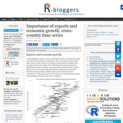
The relationship between exports’ importance in an economy and economic growth forms a good start as it is of considerable theoretical and practical policy interest and has fairly reliable time series data for many countries. At the most basic level, there is a well known positive relationship between these two variables: The relationship is made particularly strong by the small, rich countries in the top right corner. Larger countries, with their own large domestic markets, can flourish economically while being less exports-dependent than smaller countries – the USA being the example par excellence.
Create ARIMA time series from bottom up. Generating an arbitrary Auto-Regressive Integrated Moving Average (ARIMA) model is easy in R with the arima.sim() function that is part of the built-in {stats} package.
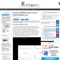
In fact I’ve done it extensively in previous blog posts for various illustrative purposes. But one cost of doing this for educational purposes is that the mechanics of generating them are hidden from the user (of course, that’s the point!). As was the case in last week’s post, I’m motivated by teaching purposes. I wanted to show people how an ARIMA model can be created, with high school maths and no special notation, from white noise. The movie that is (hopefully) playing above shows this. One interesting thing is how the AR(1) and ARMA(1, 1) models look almost identical, except for the larger variance of the ARMA(1, 1) model which comes from throwing into the mix 80% of the last period’s randomness. Reading Financial Time Series Data with R. By Joseph Rickert In a recent post focused on plotting time series with the new dygraphs package, I did not show how easy it is to read financial data into R.
However, in a thoughtful comment to the post, Achim Zeileis pointed out a number of features built into the basic R time series packages that everyone ought to know. In this post, I will just elaborate a little on what Achim sketched out. First off, I began the previous post with url strings that point to stock data for IBM and LinkedIn. Yahoo Finance make this sort of thing easy. If you already have the download URLs ibm_url and lnkd_url, then you can also simply use zoo::read.zoo() and merge the resulting closing prices: library("zoo") z <- merge( ibm = read.zoo(ibm_url, header = TRUE, sep = ",")$Close, lnkd = read.zoo(lnkd_url, header = TRUE, sep = ",")$Close )
Plotting Time Series in R using Yahoo Finance data. By Joseph Rickert I recently rediscovered the Timely Portfolio post on R Financial Time Series Plotting.
If you are not familiar with this gem, it is well-worth the time to stop and have a look at it now. Not only does it contain some useful examples of time series plots mixing different combinations of time series packages (ts, zoo, xts) with multiple plotting systems (base R, lattice, etc.) but it provides an instructive, historical perspective that illustrates the non linear nature of progress in software development: new code is written to solve certain technical problems with the current software. Progress is made, and the new code makes it possible to do some things that couldn't be done before, but there were tradeoffs. Arima. X13-SEATS-ARIMA as an automated forecasting tool.
Forecasting: principles and practice. Welcome to our online textbook on forecasting.

This textbook is intended to provide a comprehensive introduction to forecasting methods and to present enough information about each method for readers to be able to use them sensibly. We don’t attempt to give a thorough discussion of the theoretical details behind each method, although the references at the end of each chapter will fill in many of those details.
The book is written for three audiences: (1) people finding themselves doing forecasting in business when they may not have had any formal training in the area; (2) undergraduate students studying business; (3) MBA students doing a forecasting elective. We use it ourselves for a second-year subject for students undertaking a Bachelor of Commerce degree at Monash University, Australia. For most sections, we only assume that readers are familiar with algebra, and high school mathematics should be sufficient background. Use the table of contents on the right to browse the book. Time series analysis with R: Testing stuff with NetAtmo data. I’ve got a NetAtmo weather station.
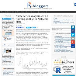
One can download the measurements from its web interface as a CSV file. I wanted to give time series analysis with the extraction of seasonal components (‘decomposition’) a try, so I thought it would be a good opportunity to use the temperature measurements of my weather station. The data is available.To make things visually a little easier, I only tried this with 14 days of temperature measurements, including all measurements from November 1st, 2015 till November 14th, 2015.The raw data looks like this (on the x-axis, there is a running number of measurements):data <- read.table(“temps.csv”, header = T, sep = “t”)plot(data$temp, type = “l”, bty = “n”, ylab = “Temperature in °C”) Don’t be too confused about the one peak over thirty degrees – we got a particularly friendly November and sometimes, the outdoor sensor of the station is standing in the sun.
Back to business.