Earth

The oxygenation of the atmosphere and oceans. Abstract The last 3.85 Gyr of Earth history have been divided into five stages.

During stage 1 (3.85–2.45 Gyr ago (Ga)) the atmosphere was largely or entirely anoxic, as were the oceans, with the possible exception of oxygen oases in the shallow oceans. During stage 2 (2.45–1.85 Ga) atmospheric oxygen levels rose to values estimated to have been between 0.02 and 0.04 atm. The shallow oceans became mildly oxygenated, while the deep oceans continued anoxic. Stage 3 (1.85–0.85 Ga) was apparently rather ‘boring’. Stage 4 (0.85–0.54 Ga) saw a rise in atmospheric oxygen to values not much less than 0.2 atm.

Climate

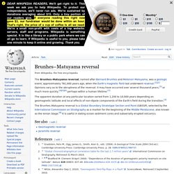
File:Timeline evolution of life.svg. Brunhes–Matuyama reversal. The apparent duration at any particular location varied from 1,200 to 10,000 years depending on geomagnetic latitude and local effects of non-dipole components of the Earth's field during the transition.[3] The Brunhes–Matuyama reversal is a Global Boundary Stratotype Section and Point (GBSSP), selected by the International Commission on Stratigraphy as a marker for the beginning of the Middle Pleistocene, also known as the Ionian Stage.[8] It is useful in dating ocean sediment cores and subaerially erupted volcanics.

See also[edit] References[edit] Jump up ^ Gradstein, Felix M.; Ogg, James G.; Smith, Alan G., eds. (2004). A Geological Time Scale 2004 (3rd ed.). Further reading[edit] Behrendt, J.C., Finn, C., Morse, L., Blankenship, D.D. Berkeley Earth. The datasets presented here have been divided into three categories: Output data, Source data, and Intermediate data.

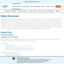
The Berkeley Earth averaging process generates a variety of Output data including a set of gridded temperature fields, regional averages, and bias-corrected station data. Source data consists of the raw temperature reports that form the foundation of our averaging system. Source observations are provided as originally reported and will contain many quality control and redundancy issues. Intermediate data is constructed from the source data by merging redundant records, identifying a variety of quality control problems, and creating monthly averages from daily reports when necessary. The definitive repository for Source and Intermediate data is located in the SVN, which is built nightly. Time Series Data Land Only (1750 – Recent) Berkeley Earth’s primary product is an analysis of summary air temperatures over land. Land + Ocean (1850 – Recent) Gridded Data. Oligocene. The Oligocene is often considered an important time of transition, a link between the archaic world of the tropical Eocene and the more modern ecosystems of the Miocene.[4] Major changes during the Oligocene included a global expansion of grasslands, and a regression of tropical broad leaf forests to the equatorial belt.

The start of the Oligocene is marked by a notable extinction event called the Grande Coupure; it featured the replacement of European fauna with Asian fauna, except for the endemic rodent and marsupial families. By contrast, the Oligocene–Miocene boundary is not set at an easily identified worldwide event but rather at regional boundaries between the warmer late Oligocene and the relatively cooler Miocene.

Subdivisions[edit] Oligocene faunal stages from youngest to oldest are: Climate[edit] The Paleogene period general temperature decline is interrupted by an Oligocene 7 million year stepwise climate change. NASA Science. Wildflower Identification. The Limits of the Earth, Part 2: Expanding the Limits. This is part two of a two-part series on the limits of human economic growth on planet Earth.

Part one details some of the environmental and natural resource challenges we’re up against. Part two, here, looks at the ultimate size of the resource pool and solutions to our problems. Both parts are based on Ramez Naam’s new book, The Infinite Resource: The Power of Ideas on a Finite Planet. Youtube. Magnetic stripes and isotopic clocks [This Dynamic Earth, USGS]

Oceanographic exploration in the 1950s led to a much better understanding of the ocean floor.

Among the new findings was the discovery of zebra stripe-like magnetic patterns for the rocks of the ocean floor. These patterns were unlike any seen for continental rocks. Obviously, the ocean floor had a story to tell, but what? In 1962, scientists of the U.S. Naval Oceanographic Office prepared a report summarizing available information on the magnetic stripes mapped for the volcanic rocks making up the ocean floor. An observed magnetic profile (blue) for the ocean floor across the East Pacific Rise is matched quite well by a calculated profile (red) based on the Earth's magnetic reversals for the past 4 million years and an assumed constant rate of movement of ocean floor away from a hypothetical spreading center (bottom).

A team of U.S. Other commonly used isotopic clocks are based on radioactive decay of certain isotopes of the elements uranium, thorium, strontium, and rubidium. How One Woman's Discovery Shook the Foundations of Geology. This story originally appeared in print in the December 2014 issue of mental_floss magazine.

Subscribe to our print edition here, and our iPad edition here. By Brooke Jarvis Marie Tharp spent the fall of 1952 hunched over a drafting table, surrounded by charts, graphs, and jars of India ink.