
NCO 4.6.1-alpha01 User Guide. This file documents NCO, a collection of utilities to manipulate and analyze netCDF files.
Copyright © 1995–2016 Charlie Zender This is the first edition of the NCO User Guide, and is consistent with version 2 of texinfo.tex. Permission is granted to copy, distribute and/or modify this document under the terms of the GNU Free Documentation License, Version 1.3 or any later version published by the Free Software Foundation; with no Invariant Sections, no Front-Cover Texts, and no Back-Cover Texts.
The license is available online at The original author of this software, Charlie Zender, wants to improve it with the help of your suggestions, improvements, bug-reports, and patches. Table of Contents. Getting started with NetCDF – reading CEH GEAR. Last year CEH released an interpolated precipitation dataset for the UK call GEAR.
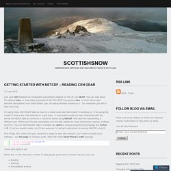
You can read about this dataset here, or view slides presented at the 2014 BHS Symposium here. In short; these data describe precipitation over Great Britain (yes, excluding Northern Ireland) at a 1 km resolution grid with a daily time step. Raster 05: Raster Time Series Data in R – NEON Work With Data. Authors: Leah A.
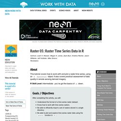
Wasser, Megan A. Jones, Zack Bryn, Kristina Riemer, Jason Williams, Jeff Hollister, Mike Smorul Reviewers: About. Time series analysis with pandas. Part 2. RasterVis. The function terrain from raster provides the vector field (gradient) from a scalar field stored in a RasterLayer object.
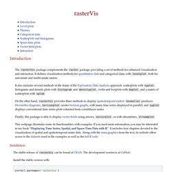
The magnitude (slope) and direction (aspect) of the vector field is usually displayed with a set of arrows (e.g. quiver in Matlab). rasterVis includes a method, vectorplot, to calculate and display this vector field. proj <- CRS('+proj=longlat +datum=WGS84') df <- expand.grid(x = seq(-2, 2, .01), y = seq(-2, 2, .01)) df$z <- with(df, (3*x^2 + y)*exp(-x^2-y^2)) r <- rasterFromXYZ(df, crs=proj) vectorplot(r, par.settings=RdBuTheme()) Raster02. Map and analyze raster data in R. The amount of spatial analysis functionality in R has increased dramatically since the first release of R. In a previous post, for example, we showed that the number of spatial-related packages has increased to 131 since the first R release. This means, of course, that more and more of your spatial-related workflow can be conducted without leaving R.
Extracting Climate Data in R - Creative morphometrics. With the ongoing expand of the available geospatial databases in raster format (GeoTiff) it is getting easier to analyse the relationship between any complex morphology, captured in landmark data, and i.e. climate or precipitation data with the help of partial least squares (PLS).
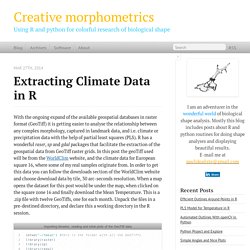
R has a wonderful raser, sp and gdal packages that facilitate the extraction of the geospatial data from GeoTiff raster grids. In this post the geoTiff used will be from the WorldClim website, and the climate data for European square 16, where some of my real samples originate from. In order to get this data you can follow the downloads section of the WorldClim website and choose download data by tile, 30 arc-seconds resolution. Geospatial Data Processing and Analysis in R. Multiple plots in one page.
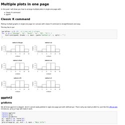
In this post I will show you how to arrange multiple plots in single one page with: Classic R commandggplot.
SpatialAnalysisTutorials/CDO_Process.md at master · adammwilson/SpatialAnalysisTutorials. Plotting a map of NetCDF data with Matplotlib/Basemap – Water Programming: A Collaborative Research Blog. In two previous posts I showed how to create a NetCDF file from a mess of ASCII data, and how to reduce its size by storing only the lat-lon grid cells for which data exists.
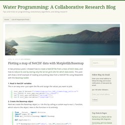
This post will show a brief example of reading and plotting data from a NetCDF file using Matplotlib with the Basemap toolkit. 1. Read in NetCDF variables This is an easy one—just open the file and assign the values you want to plot. 2. Create the Basemap object Next we create the Basemap object, m. I did this because I wanted to modularize the projection and color scheme that I found to look “nice” for plotting global data. Spatial data in R: Using R as a GIS. Plotting netCDF data with Python — Hydro-Logic. How to Read Data in netCDF Format with R. A3. Advanced notes: Scientific and Numerical Python — GeogG122: Scientific Computing v<release> documentation.
A3.1 Pulling Compressed netCDF Files Sometimes, such as when we want to pull data from netCDF files from some data site such as we might find that ‘older style’ formats have been used, such as netCDF3 which might not have internal compression.
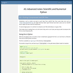
To save storage space, it is common to compress such files extrenally (i.e. to gzip a file). That makes direct reading from a url a bit more tricky, and in such cases, we may as well uncompress the file to a local temporary file. Visualizing netcdf panoply. NetCDF in R. NetCDF is a self-documenting, machine-independent format for creating and distributing arrays of gridded data.
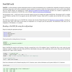
Originally developed for storing and distributing climate data, such as those generated by climate simulation or reanalysis models, the format and protocols can be used for other gridded data sets. netCDF libraries are maintained by Unidata and there are a number of applications for producing simple visualizations of NetCDF files, such as Panoply, The R packages ncdf, ncdf4 and raster provide the support necessary for reading and writing NetCDF files. The package ncdf is available on both Windows and Mac OS X, but supports only the older NetCDF 3 formats, while ncdf4 is available only for the Mac OS X (as of May 2013). Examples — pytesmo 0.3.5 documentation. Reading the H08 product¶ H08 data has a much higher resolution and comes on a 0.00416 degree grid.
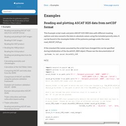
The sample data included in pytesmo was observed on the same time as the included H07 product. Loading Data and Basic Formatting in R. Oftentimes, the bulk of the work that goes into a visualization isn't visual at all. That is, the drawing of shapes and colors can be relatively quick, and you might spend most of your time getting the data in the format that you need (or just getting data in general). This can be especially frustrating when you have your data, you know what you want to make, but you're stuck in the middle. This tutorial covers the basics of getting your data into R so that you can move on to more interesting things. Setup Since this is in R, you need to install the free statistical computing language on your computer. That's it. You can either use the setwd() function or you can change your working directory via the Misc > Change Working Directory... menu.
Working%20with%20Time%20Series%20Data%20in%20R. Documentation and Examples. A Compendium of Clean Graphs in R. R: Hydrological time series plotting and extraction. Advanced Plotting Capability of "R" Introduction The main aim of this article is to show the advanced graphical capability of R. Once you get the primary knowledge about basic functions and plotting pattern, you can easily generate complex graphs just writing some commands. Claudia @ work. This is the third of a series of tutorials on the FUSE implementation within the RHydro package. The script for this tutorial is available here. If you are interested in following the discussion related to this post and see how it evolves, join the R4Hydrology community on Google+! If you want to know what FUSE is, how to prepare your data and run a simple simulation go to the first post of the series, while for a basic calibration example (using 1 model structure) go to the second post.
Recap from previous posts. NCL Tutorial V1.1. Plot multiple lines (data series) each with unique color in R. Python Programming Tutorials. KL worksheet2a.