
R - Generalized linear Models. 5 Generalized Linear Models Generalized linear models are just as easy to fit in R as ordinary linear model.
In fact, they require only an additional parameter to specify the variance and link functions. 5.1 Variance and Link Families The basic tool for fitting generalized linear models is the glm function, which has the folllowing general structure: > glm(formula, family, data, weights, subset, ...) where ... stands for more esoteric options.
As can be seen, each of the first five choices has an associated variance function (for binomial the binomial variance m(1-m)), and one or more choices of link functions (for binomial the logit, probit or complementary log-log). As long as you want the default link, all you have to specify is the family name. Exposure as a possible explanatory variable. Iin insurance pricing, the exposure is usually used as an offset variable to model claims frequency.

As explained many times on this blog (e.g. here), and in my notes, if we have to identical drivers, but one with an exposure of 6 months, and the other one of one year, it should be natural to assume that, on average, the second driver will have two times more accidents. Poisson regression fitted by glm(), maximum likelihood, and MCMC. The goal of this post is to demonstrate how a simple statistical model (Poisson log-linear regression) can be fitted using three different approaches.

I want to demonstrate that both frequentists and Bayesians use the same models, and that it is the fitting procedure and the inference that differs. This is also for those who understand the likelihood methods and do not have a clue about MCMC, and vice versa. I use an ecological dataset for the demonstration. The complete code of this post is available here on GitHub The data I will use the data on the distribution of 3605 individual trees of Beilschmiedia pendula in 50-ha (500 x 1000 m) forest plot in Barro Colorado (Panama).
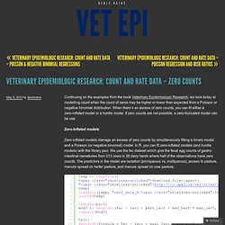
Vet Epi Research: Count and Rate Data – Poisson Regression and Risk Ratios. Vet Epi Research: Count and Rate Data – Zero Counts. Continuing on the examples from the book Veterinary Epidemiologic Research, we look today at modelling count when the count of zeros may be higher or lower than expected from a Poisson or negative binomial distribution.
Logistic - Poisson regression to estimate relative risk for binary outcomes. Re: st: offset variables. Interpretation of intercept term in poisson model with offset and covariates. Specification and interpretation of interaction terms using glm() A minor update to simstudy provides an excuse to talk a bit about the negative binomial and Poisson distributions. I just updated simstudy to version 0.1.5 (available on CRAN) so that it now includes several new distributions - exponential, discrete uniform, and negative binomial.
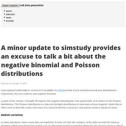
As part of the release, I thought I’d explore the negative binomial just a bit, particularly as it relates to the Poisson distribution. The Poisson distribution is a discrete (integer) distribution of outcomes of non-negative values that is often used to describe count outcomes. It is characterized by a mean (or rate) and its variance equals its mean. Added variation In many situations, when count data are modeled, it turns out that the variance of the data exceeds the mean (a situation called over-dispersion). We can see this by generating data from each distribution with mean 15, and a dispersion parameter of 0.2 for the negative binomial. Underestimating standard errors In this simple simulation, we generate two predictors (\(x\) and \(b\)) and an outcome (\(y\)). Risk Ratio vs Rate Ratio. Lead Author(s): Jeff Martin, MD Relative risk or RR is very common in the literature, but may represent: There can be substantial difference in the association of a risk factor with prevalent disease versus incident disease In the general medical literature, rate is often incorrectly used for prevalence measures.

These inconsistencies are even greater and are compounded by the fact that an abbreviation for both a risk ratio and a rate ratio is RR. Often RR is used to mean relative risk, which is taken loosely to include several different ratio measures. Confidence intervals for GLMs. You've estimated a GLM or a related model (GLMM, GAM, etc.) for your latest paper and, like a good researcher, you want to visualise the model and show the uncertainty in it.

In general this is done using confidence intervals with typically 95% converage. If you remember a little bit of theory from your stats classes, you may recall that such an interval can be produced by adding to and subtracting from the fitted values 2 times their standard error. Unfortunately this only really works like this for a linear model. If I had a dollar (even a Canadian one) for every time I've seen someone present graphs of estimated abundance of some species where the confidence interval includes negative abundances, I'd be rich!
Here, following the rule of "if I'm asked more than once I should write a blog post about it! " Why is plus/minus two standard errors wrong? Well, it's not! Rare disease assumption. The rare disease assumption is a mathematical assumption in epidemiologic case-control studies where the hypothesis tests the association between an exposure and a disease.

It is assumed that, if the prevalence of the disease is low, then the odds ratio approaches the relative risk. Case control studies are relatively inexpensive and less time consuming than cohort studies. [citation needed] Since case control studies don't track patients over time, they can't establish relative risk. The case control study can, however, calculate the exposure-odds ratio, which, mathematically, is supposed to approach the relative risk as prevalence falls. Some authors[who?] The following example will illustrate this difficulty clearly. Unable to test linearity assumption of logistic regression. At 02:52 AM 6/23/2006, Benoît Depaire wrote: >I am doing a simple binary logistic regression >with the following structure: > >logit(Y) = a + bX > >X is a categorical variable with 5 categories, >which is entered into the model as indicator >[variables] with the last category as reference.
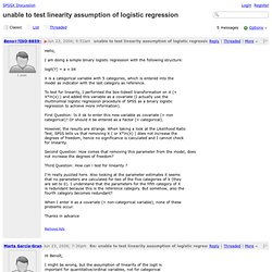
> >To test for linearity, I performed the >box-tidwell transformation on X (=X*ln(x) ) and >added this variable as a covariate. Curious: what does the transformation mean, if X is a categorical variable? If it's truly categorical, it would be the same variable after any RECODE, like but that would raise Cain with the transformation, wouldn't it? Or, what if the categories were A, B, C, D and E? >The results are strange. Exactly. Obtaining predicted values (Y=1 or 0) from a logistic regression model fit. Glm.fit: "fitted probabilities numerically 0 or 1 occurr. What is complete or quasi-complete separation in logistic/probit regression and how do we deal with them?
Occasionally when running a logistic/probit regression we run into the problem of so-called complete separation or quasi-complete separation.
On this page, we will discuss what complete or quasi-complete separation is and how to deal with the problem when it occurs. R - How to deal with perfect separation in logistic regression? Seeking a Theoretical Understanding of Firth Logistic Regression. R - Evaluating a binomial (success vs. failure) glm. A pathological glm() problem that doesn’t issue a warning. Vet Epi Research: GLM (part 4) – Exact and Conditional Logistic Regressions.
Beta distribution GLM with categorical independents and proportional response. How to interpret the coefficients from a beta regression? Why is the standard error different in these two fitting methods (R Logistic Regression and Beta Regression) for a common dataset?