
How to Use the VLOOKUP HLOOKUP Combination Formula – MBA Excel. VLOOKUP and HLOOKUP are two of the most popular formulas in Excel and using them together is one of the first formula combinations that people learn.
While using INDEX MATCH for vertical lookups and INDEX MATCH MATCH for matrix style lookups are superior approaches, it’s still a good idea to learn this formula combination and add it to your toolkit of lookup approaches. You may find yourself in a situation where you encounter this formula combination after inheriting someone else’s file, or you may just be working with someone who does not understand INDEX MATCH. Both of these contexts make it worthwhile to learn VLOOKUP HLOOKUP. Objective and When to Use There are two key requirements for using VLOOKUP HLOOKUP.
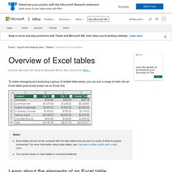
Your data table needs to have lookup values on both the top and left hand side. In the example below, we have Country as a potential lookup value down the leftmost column and Year as a lookup value across the headings at the top. The Syntax. Overview of Excel tables. To make managing and analyzing a group of related data easier, you can turn a range of cells into an Excel table (previously known as an Excel list).
Notes: Excel tables should not be confused with the data tables that are part of a suite of what-if analysis commands. For more information about data tables, see Calculate multiple results with a data table. Create a PivotChart. To create a PivotChart on the Mac, you need to create a PivotTable first, and then insert a chart.
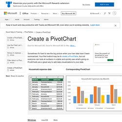
Once that is done, the chart will behave like a PivotChart if you change the fields in the PivotTable Fields list. Create a PivotTable if you don't have one already. Select any cell within the PivotTable. On the Insert tab, click a button to insert either a column, line, pie, or radar chart. Please note that other types of charts do not work with PivotTables at this time. Sort data in a PivotTable or PivotChart. Follow these steps to sort in Excel Desktop: In a PivotTable, click the small arrow next to Row Labels and Column Labels cells.
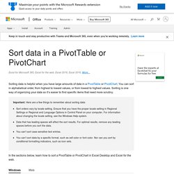
Click a field in the row or column you want to sort. Click the arrow on Row Labels or Column Labels, and then click the sort option you want. To sort data in ascending or descending order, click Sort A to Z or Sort Z to A. Text entries will sort in alphabetical order, numbers will sort from smallest to largest (or vice versa), and dates or times will sort from oldest to newest (or vice versa). Overview of PivotTables and PivotCharts. If you are familiar with standard charts, you will find that most operations are the same in PivotCharts.
However, there are some differences: Video: Advanced IF functions. Before we get started with advanced IF functions, let's do a quick IF function refresher first.
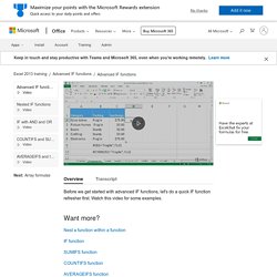
Watch this video for some examples. Want more? IFS function. The IFS function checks whether one or more conditions are met, and returns a value that corresponds to the first TRUE condition.
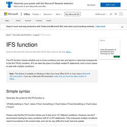
IFS can take the place of multiple nested IF statements, and is much easier to read with multiple conditions. Simple syntax Generally, the syntax for the IFS function is: =IFS([Something is True1, Value if True1,Something is True2,Value if True2,Something is True3,Value if True3) Please note that the IFS function allows you to test up to 127 different conditions. Technical details. SUBTOTAL function. This article describes the formula syntax and usage of the SUBTOTAL function in Microsoft Excel.
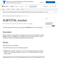
Description Returns a subtotal in a list or database. It is generally easier to create a list with subtotals by using the Subtotal command in the Outline group on the Data tab in the Excel desktop application. Once the subtotal list is created, you can modify it by editing the SUBTOTAL function. Syntax SUBTOTAL(function_num,ref1,[ref2],...) The SUBTOTAL function syntax has the following arguments: Function_num Required. Remarks. Using structured references with Excel tables. When you create an Excel table, Excel assigns a name to the table, and to each column header in the table.
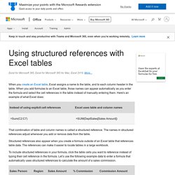
When you add formulas to an Excel table, those names can appear automatically as you enter the formula and select the cell references in the table instead of manually entering them. Here's an example of what Excel does: That combination of table and column names is called a structured reference. Overview of Excel tables. Available chart types in Office. For a description of each chart type, select an option from the following drop-down list.
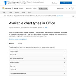
Excel for Windows training. Microsoft 365 basics video training - Office 365. Create a chart from start to finish. Note: Some of the content in this topic may not be applicable to some languages. Charts display data in a graphical format that can help you and your audience visualize relationships between data. When you create a chart, you can select from many chart types (for example, a stacked column chart or a 3-D exploded pie chart). After you create a chart, you can customize it by applying chart quick layouts or styles. Learn the elements of a chart Charts contain several elements, such as a title, axis labels, a legend, and gridlines. Chart title Plot area Legend Axis titles Axis labels Tick marks. How to avoid broken formulas. Don't enter numbers formatted with dollar signs ($) or decimal separators (,) in formulas, because dollar signs indicate Absolute References and commas are argument separators.
Instead of entering $1,000, enter 1000 in the formula. If you use formatted numbers in arguments, you’ll get unexpected calculation results, but you may also see the #NUM! Error. For example, if you enter the formula =ABS(-2,134) to find the absolute value of -2134, Excel shows the #NUM! Error, because the ABS function accepts only one argument, and it sees the -2, and 134 as separate arguments.
Note: You can format the formula result with decimal separators and currency symbols after you enter the formula using unformatted numbers (constants). Overview of formulas in Excel. Guidelines and examples of array formulas. This section provides examples of advanced array formulas. Create a chart from start to finish. Overview of formulas in Excel.