
Removing #NA or #Value in Index Match Formuals. Excel University. Of all the functions introduced in Excel 2007, 2010, and 2013, my personal favorite is SUMIFS.
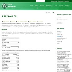
The SUMIFS function performs multiple condition summing. The function is designed with AND logic, but, there are several techniques that allow us to use OR logic instead. This post explores a few of them. Objective Let’s be clear about our objective by taking a look at a worksheet. We want to populate the report by aggregating the values from the exported accounting data, shown below. Since the SUMIFS function is designed with AND logic, the following formula wouldn’t work to populate the report’s sales value: =SUMIFS($C$18:$C$28, $B$18:$B$28,"Sales-Labor", $B$18:$B$28,"Sales-Hardware", $B$18:$B$28,"Sales-Software") The formula wouldn’t work because there are no rows where the account is equal to Sales-Labor AND equal to Sales-Hardware AND equal to Sales-Software.
Now that we have a clear idea of the situation, let’s work through several approaches. SUMIFS and Wildcard. How to remove blank or empty rows in Excel? If there are hundreds of blank rows scattering through the whole worksheets, you will be frustrated about it.
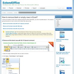
This tutorial is giving instructions on how to remove all the blank rows step by step. Remove all the blank rows with Go To Special command Remove all the blank rows with VBA code Remove all the blank rows with only one click. How to fill blank cells with value above in Excel? When we set up data in Excel, we always leave a blank cell if the data for that cell is the same as the cell above.
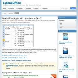
For example, I have a worksheet such as the following screenshot: This form looks neater and nicer if there is just one header row instead of lots of repeated rows. Excel Lookup Formula with Multiple Criteria. Create combination stacked / clustered charts in Excel. How to Combine Stacked and Clustered Charts in Excel. Tips & tricks for better looking Charts in Excel 2010, 2013, 2007. Some tips, tricks and techniques for better looking charts in Microsoft Excel.

The charting tools in Microsoft Excel 2010 and 2007 are way better in looks and functionality from those that were available in earlier Excel versions. While the charts look better, not all the options you can use to make them more functional are immediately apparent. Unlinking A Pivot Table From Its Source Data. Category: General / Formatting | [Item URL] You may have a situation in which you need to send someone a pivot table summary report, but you don't want to include the original data.
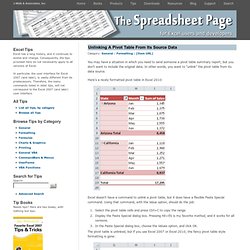
In other words, you want to "unlink" the pivot table from its data source. Here's a nicely formatted pivot table in Excel 2010: Excel doesn't have a command to unlink a pivot table, but it does have a flexible Paste Special command. Using that command, with the Value option, should do the job: Utility20/Documentation20/Using_the_Peltier_Tech_Utility.pdf. Peltier Tech Chart Utility for Excel. There is a new version of this software.
Go to Peltier Tech Charts for Excel 3.0 for information. Purchase the Peltier Tech Chart Utility Advanced Edition Excel 2007, 2010, 2013for Windows. Standard Edition Excel 2011 forMacintosh. View Cart General Features of the Peltier Tech Chart Utility Excel 2007, 2010, and 2013 for Windows (32-bit and 64-bit). Clustered and Stacked Column and Bar Charts. Excel has built-in chart types for clustered columns and bars, and for stacked columns and bars.
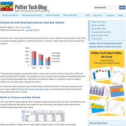
One of the commonest charting questions in online Excel forums is, “How do I make a chart that is both clustered and stacked?” This article demonstrates a protocol that works in both modern versions of Excel, that is, Excel 2003 and earlier and Excel 2007 and later. The technique is a bit convoluted, and it requires an expanded data layout to get the appropriate appearance. And there’s an additional degree of complexity to get the category labels to line up neatly under or beside the clusters. Jon's Excel Charts and Tutorials - Index. What to do when Excel won't let you insert columns. By David H.

Clustered and stacked bar charts in excel. Possible! Check Multiple Criteria with Excel INDEX and MATCH. The INDEX function can return a value from a range of cells, and the MATCH function can calculate a value's position in a range of cells.
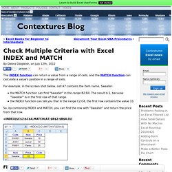
For example, in the screen shot below, cell A7 contains the item name, Sweater: the MATCH function can find "Sweater" in the range B2:B4. The result is 1, because "Sweater" is in the first row of that range.the INDEX function can tell you that in the range C2:C4, the first row contains the value 10. So, by combining INDEX and MATCH, you can find the row with "Sweater" and return the price from that row. Find a Match for Multiple Criteria In the previous example, the match was based solely on the Item name – Sweater.
In the screen shot below, each item is listed 3 times in the pricing lookup table. Does it MATCH? Instead of a simple MATCH formula, we'll use one that checks both the Item and Size columns. If the Item in column B is a Jacket, the result in column E is TRUE. Use MATCH With Multiple Criteria In this example, More INDEX and MATCH Examples. How do I get countifs to select all non-blank cells in Excel. Round number so they are divisible by six. Remove spaces from the beginning and end of a cell. Important notice for users of Office 2003 To continue receiving security updates for Office, make sure you're running Office 2003 Service Pack 3 (SP3).
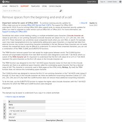
The support for Office 2003 ends April 8, 2014. If you’re running Office 2003 after support ends, to receive all important security updates for Office, you need to upgrade to a later version such as Office 365 or Office 2013. For more information, see Support is ending for Office 2003. Sometimes text values contain leading, trailing, or multiple embedded space characters (Unicode character set (Unicode: A character encoding standard developed by the Unicode Consortium.
By using more than one byte to represent each character, Unicode enables almost all of the written languages in the world to be represented by using a single character set.) values 32 and 160), or non-printing characters (Unicode character set values 0 to 31, 127, 129, 141, 143, 144, and 157). Data Cleanup Tips for Microsoft Excel. Access ¨ Excel ¨ FrontPage ¨ Outlook ¨ PowerPoint ¨ Word ¨ Miscellaneous ¨ Tutorials ¨ Windows ¨ Free Downloads I have been cleaning up data files in Microsoft Excel for a very long time. This article will likely always be a work in process, so check back any time you have a data cleanup job to do. Or email us to let us know a task you'd like us to include here. Data Isn't Recognized Properly You add up a column of data, and you get zero, or anything but the right result. To force Excel to see your numeric values properly, just perform some arithmetic on them.
Having hidden rows and columns can also provide unexpected results. Clean Up Extra Spaces or Characters Using Find and Replace This is simple; it just takes a series of tasks. To get rid of spaces within cells. Find what: Type 2 spaces using the spacebar Replace with: Type 1 space using the spacebar Replace all. How do I insert a line in an area chart in MS Excel.
Add a Horizontal Line to a Column or Line Chart: Error Bar Method. How do you add a nice vertical line to a column or line chart, to show a target value, or the series average? The method involves adding a new one-point series with an error bar, applying it to the secondary axes, and making the secondary axes disappear. Straight lines. There are many instances when one needs to add a visual indicator to a chart. This could be a line indicating a goal of some sort. Or, it could be a line showing the average of the graphed data. In TQM control charts, it could be a line so-many standard deviations from the mean. Excel Constant horizontal line on a chart (based on a single value) Back to Charting for Excel archive indexBack to archive home Constant horizontal line on a chart (based on a single value) Posted by Skewer on July 18, 2001 11:22 AM Image the scene, you want a graph showing stuff but there is an ideal value or range of values (as in cost, weight, etc).
How can I get a single value (already calculated elsewhere) or values to generate horizontal lines so at a glance the approach towards (or fluctuation between) certain values is visible?