
Data transformation in #tidyverse style: package sjmisc updated #rstats – Strenge Jacke! I’m pleased to announce an update for the sjmisc-package, which was just released on CRAN.
Here I want to point out two important changes in the package. New default option for recoding and transformation functions First, a small change in the code with major impact on the workflow, as it affects argument defaults and is likely to break your existing code – if you’re using sjmisc: The append-argument in recode and transformation functions like rec(), dicho(), split_var(), group_var(), center(), std(), recode_to(), row_sums(), row_count(), col_count() and row_means() now defaults to TRUE. The reason behind this change is that, in my experience and workflow, when transforming or recoding variables, I typically want to add these new variables to an existing data frame by default.
Especially in a pipe-workflow, when I start my scripts with importing and basic tidying of my data, I almost always want to append the recoded variables to my existing data, e.g. Package sjstats. Collection of convenient functions for common statistical computations, which are not directly provided by R's base or stats packages.
This package aims at providing, first, shortcuts for statistical measures, which otherwise could only be calculated with additional effort (like standard errors or root mean squared errors). Second, these shortcut functions are generic (if appropriate), and can be applied not only to vectors, but also to other objects as well (e.g., the Coefficient of Variation can be computed for vectors, linear models, or linear mixed models; the r2()-function returns the r-squared value for 'lm', 'glm', 'merMod' or 'lme' objects). The focus of most functions lies on summary statistics or fit measures for regression models, including generalized linear models and mixed effects models. However, some of the functions also deal with other statistical measures, like Cronbach's Alpha, Cramer's V, Phi etc. Package sjmisc. Beautiful tables for linear model summaries #rstats.
In this blog post I’d like to show some (old and) new features of the sjt.lm function from my sjPlot-package.
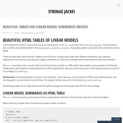
These functions are currently only implemented in the development snapshot on GitHub. A package update is planned to be submitted soon to CRAN. There are two new major features I added to this function: Comparing models with different predictors (e.g. stepwise regression) and automatic grouping of categorical predictors. There are examples below that demonstrate these features. The sjt.lm function prints results and summaries of linear models as HTML-table. Please note: The following tables may look a bit cluttered – this is because I just pasted the HTML-code created by knitr into this blog post, so style sheets may interfere. SjPlot package and related online manuals updated #rstats # ggplot. My sjPlot package for data visualization has just been updated on CRAN.
I’ve added some features to existing function, which I want to introduce here. Plotting linear models So far, plotting model assumptions of linear models or plotting slopes for each estimate of linear models were spread over several functions. Now, these plot types have been integrated into the sjp.lm function, where you can select the plot type with the type parameter. Furthermore, plotting standardized coefficients now also plot the related confidence intervals. Detailed examples can be found here:www.strengejacke.de/sjPlot/sjp.lm.
SjPlot: New options for creating beautiful tables, documentation on #RPubs #rstats. SjPlot 1.3 available #rstats #sjPlot. I just submitted my package update (version 1.3) to CRAN.
The download is already available (currently source, binaries follow). While the last two updates included new functions for table outputs (see here and here for details on these functions), the current update mostly provides small helper functions. The focus of this update was to improve existing functions and make their handling easier and more comfortable. Automatic label detection One major feature is that many functions now automatically detect variables and value labels, if possible. But what are the exactly the benefits of this new feature? Since version 1.3, you only need to write: Reliability check for index scores One new table output function included in this update is sjt.itemanalysis, which helps performing an item analysis on a scale or data frame if you want to develop index scores. The output of the computed PCA was suppressed by no.output=TRUE. The latest developer build can be found on github. Beautiful table outputs in R, part 2 #rstats #sjPlot.
First of all, I’d like to thank my readers for the lots of feedback on my last post on beautiful outputs in R.
I tried to consider all suggestions, updated the existing table-output-functions and added some new ones, which will be described in this post. The updated package is already available on CRAN. This posting is divided in two major parts: the new functions are described, andthe new features of all table-output-functions are introduced (including knitr-integration and office-import) First I want to give an overview of the new functions. Viewing imported SPSS data sets As I have mentioned some times before, one purpose of this package is to make it easier for (former) SPSS users to switch to and use R.
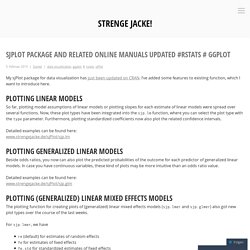
With the function sji.viewSPSS you can easily create a kind of “code plan” for your data sets. This will give you an overview of: Variable number, variable name, variable label, variable values and value labels: Description and content of data frames Stacked frequencies and Likert scales. Simply creating various scatter plots with ggplot #rstats. Inspired by these two postings, I thought about including a function in my package for simply creating scatter plots.
In my package, there’s a function called sjp.scatter for creating scatter plots. To reproduce these examples, first load the package and then attach the sample data set: The simplest function call is by just providing two variables, one for the x- and one for the y-axis: which plots following graph: If you have continuous variables with a larger scale, you shouldn’t have problems with overplotting or overlaying dots. The same plot, when auto-jittering is turned off, would look like this: You can also add a grouping variable. If the groups are difficult to distinguish in a single plot area, the graph can be faceted by groups. Find a complete overview of the various function options in the package-help or at inside-r. SjPlot. SjPlot has been released on CRAN!
You can install the package and its dependencies using install.packages("sjPlot")! Description Collection of several plotting and table output functions for data visualization. Results of several statistical analyses (that are commonly used in social sciences) can be visualized using this package, including simple and cross tabulated frequencies, histograms, box plots, (generalized) linear models (forest plots), PCA, correlations, cluster analyses, scatter plots etc. Beautiful output in R. Note: There’s a second part of this series here.
About one year ago, I seriously started migrating from SPSS to R. Though I’m still using SPSS (because I have to in some situations), I’m quite comfortable and happy with R now and learnt a lot in the past months. But since SPSS is still very wide spread in social sciences, I get asked every now and then, whether I really needed to learn R, because SPSS meets all my needs…