
Iterated function system. In mathematics, iterated function systems or IFSs are a method of constructing fractals; the resulting constructions are always self-similar.
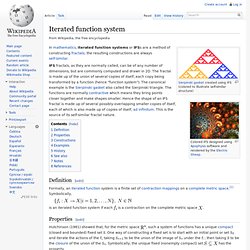
IFS fractals, as they are normally called, can be of any number of dimensions, but are commonly computed and drawn in 2D. The fractal is made up of the union of several copies of itself, each copy being transformed by a function (hence "function system"). The canonical example is the Sierpinski gasket also called the Sierpinski triangle. The functions are normally contractive which means they bring points closer together and make shapes smaller. Hence the shape of an IFS fractal is made up of several possibly-overlapping smaller copies of itself, each of which is also made up of copies of itself, ad infinitum. Definition[edit] Formally, an iterated function system is a finite set of contraction mappings on a complete metric space.[1] Symbolically, is an iterated function system if each.
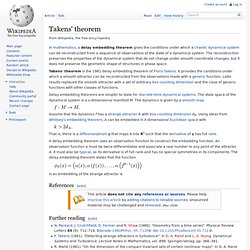
Lacunarity. Figure 1.
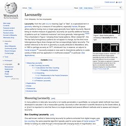
Basic fractal patterns increasing in lacunarity from left to right. The same images as above, rotated 90°. Whereas the first two images appear essentially the same as they do above, the third looks different from its unrotated original. This feature is captured in measures of lacunarity listed across the top of the figures, as calculated using standard biological imaging box counting software ImageJ (FracLac plugin). Lacunarity, from the Latin lacuna meaning "gap" or "lake", is a specialized term in geometry referring to a measure of how patterns, especially fractals, fill space, where patterns having more or larger gaps generally have higher lacunarity. Measuring Lacunarity[edit] In many patterns or data sets, lacunarity is not readily perceivable or quantifiable, so computer-aided methods have been developed to calculate it. Or but it is important to note that there is no single standard and several different methods exist to assess and interpret lacunarity.
Figure 2a. S. In vs at.
Recurrence quantification analysis. Recurrence quantification analysis (RQA) is a method of nonlinear data analysis (cf. chaos theory) for the investigation of dynamical systems.
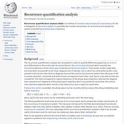
It quantifies the number and duration of recurrences of a dynamical system presented by its phase space trajectory. Background[edit] The recurrence quantification analysis was developed in order to quantify differently appearing recurrence plots (RPs) based on the small-scale structures therein. Recurrence plots are tools which visualise the recurrence behaviour of the phase space trajectory of dynamical systems. They mostly contain single dots and lines which are parallel to the mean diagonal (line of identity, LOI) or which are vertical/horizontal. If only a time series is available, the phase space can be reconstructed by using a time delay embedding (see Takens' theorem): where. Correlation integral. In chaos theory, the correlation integral is the mean probability that the states at two different times are close: where is the number of considered states is a threshold distance, a norm (e.g.
Euclidean norm) and the Heaviside step function. Takens' theorem. In mathematics, a delay embedding theorem gives the conditions under which a chaotic dynamical system can be reconstructed from a sequence of observations of the state of a dynamical system.
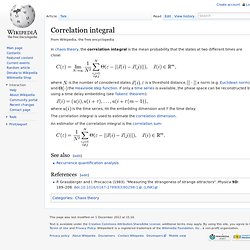
The reconstruction preserves the properties of the dynamical system that do not change under smooth coordinate changes, but it does not preserve the geometric shape of structures in phase space. Takens' theorem is the 1981 delay embedding theorem of Floris Takens. It provides the conditions under which a smooth attractor can be reconstructed from the observations made with a generic function. Later results replaced the smooth attractor with a set of arbitrary box counting dimension and the class of generic functions with other classes of functions. Delay embedding theorems are simpler to state for discrete-time dynamical systems. Assume that the dynamics f has a strange attractor A with box counting dimension dA. Is an embedding of the strange attractor A. References[edit] Further reading[edit] N. Minkowski–Bouligand dimension. Estimating the box-counting dimension of the coast of Great Britain Suppose that N(ε) is the number of boxes of side length ε required to cover the set.
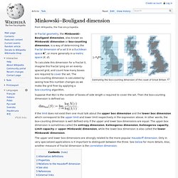
Then the box-counting dimension is defined as: If the limit does not exist then one must talk about the upper box dimension and the lower box dimension which correspond to the upper limit and lower limit respectively in the expression above. In other words, the box-counting dimension is well defined only if the upper and lower box dimensions are equal.