
Cytoscape.js. This is how easy it is to get started with Cytoscape.js (this code creates the instance you see on the bottom-right: About Cytoscape.js is an open-source graph theory library written in JavaScript.
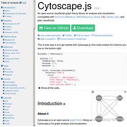
You can use Cytoscape.js for graph analysis and visualisation. Cytoscape.js allows you to easily display and manipulate rich, interactive graphs. Because Cytoscape.js allows the user to interact with the graph and the library allows the client to hook into user events, Cytoscape.js is easily integrated into your webapp, especially since Cytoscape.js supports both desktop browsers, like Chrome, and mobile browsers, like on the iPad.
Cytoscape.js also has graph analysis in mind: The library contains a slew of useful functions in graph theory. Cytoscape.js is an open-source project, and anyone is free to contribute. Cs.brown.edu/~rt/gdhandbook/chapters/force-directed.pdf. Livizjs/liviz/js at master · gyuque/livizjs. Pure JavaScript Graphviz equivalent. Glossary of graph theory. Graph theory is a growing area in mathematical research, and has a large specialized vocabulary.
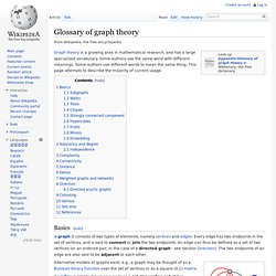
Some authors use the same word with different meanings. Some authors use different words to mean the same thing. This page attempts to describe the majority of current usage. Basics[edit] In this pseudograph the blue edges are loops and the red edges are multiple edges of multiplicity 2 and 3. An edge (a set of two elements) is drawn as a line connecting two vertices, called endpoints or (less often) endvertices.
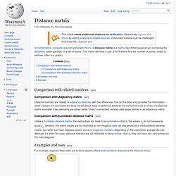
The size of a graph is the number of its edges, i.e. Graphs whose edges or vertices have names or labels are known as labeled, those without as unlabeled. (Graph labeling usually refers to the assignment of labels (usually natural numbers, usually distinct) to the edges and vertices of a graph, subject to certain rules depending on the situation. A labeled simple graph with vertex set V = {1, 2, 3, 4, 5, 6} and edge set E = {{1,2}, {1,5}, {2,3}, {2,5}, {3,4}, {4,5}, {4,6}}. and. Adjacency matrix. Distance matrix. Comparison with related matrices[edit] Comparison with Adjacency matrix[edit] Distance matrices are related to adjacency matrices, with the differences that (a) the latter only provides the information which vertices are connected but does not tell about costs or distances between the vertices and (b) an entry of a distance matrix is smaller if two elements are closer, while "close" (connected) vertices yield larger entries in an adjacency matrix.
Comparison with Euclidean distance matrix[edit] Unlike a Euclidean distance matrix, the matrix does not need to be symmetric—that is, the values xi,j do not necessarily equal xj,i. Similarly, the matrix values are not restricted to non-negative reals (as they would be in the Euclidean distance matrix) but rather can have negative values, zeros or imaginary numbers depending on the cost metric and specific use. Examples and uses[edit] Raw data The distance matrix would be: These data can then be viewed in graphic form as a heat map.
Graphical View. Trace (linear algebra) For other uses, see Trace In linear algebra, the trace of an n-by-n square matrix A is defined to be the sum of the elements on the main diagonal (the diagonal from the upper left to the lower right) of A, i.e.
Stress majorization. .
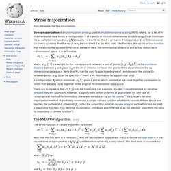
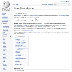
Usually r is 2 or 3, i.e. the (r x n) matrix X lists points in 2- or 3-dimensional Euclidean space so that the result may be visualised (i.e. an MDS plot). The function is a cost or loss function that measures the squared differences between ideal ( -dimensional) distances and actual distances in r-dimensional space. It is defined as: where is a weight for the measurement between a pair of points. Force-directed graph drawing. Visualization of links between pages on a wiki using a force-directed layout.
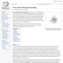
While graph drawing can be a difficult problem, force-directed algorithms, being physical simulations, usually require no special knowledge about graph theory such as planarity. Forces[edit] Barnes–Hut simulation. A 100-body simulation with the Barnes-Hut tree visually as blue boxes.

The Barnes–Hut simulation (Josh Barnes and Piet Hut) is an algorithm for performing an n-body simulation. It is notable for having order O(n log n) compared to a direct-sum algorithm which would be O(n2). The simulation volume is usually divided up into cubic cells via an octree (in a three-dimensional space), so that only particles from nearby cells need to be treated individually, and particles in distant cells can be treated as a single large particle centered at the cell's center of mass (or as a low-order multipole expansion).
This can dramatically reduce the number of particle pair interactions that must be computed. Algorithm[edit]