
Python for Signal Processing. Maximum Likelihood Estimation Maximum likelihood estimation is one of the key techniques employed in statistical signal processing for a wide variety of applications from signal detection to parameter estimation.
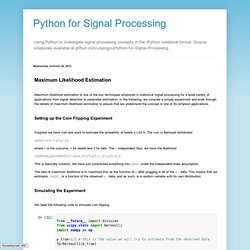
In the following, we consider a simple experiment and work through the details of maximum likelihood estimation to ensure that we understand the concept in one of its simplest applications. Setting up the Coin Flipping Experiment. How to get beautifully typeset maths on your blog. Lots of people have blogs where they talk about maths.
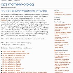
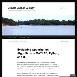
Lots of these people just use plain text for mathematical notation which, while it gets the point across, isn’t as easy to read or as visually appealing as it could be. MathJax lets you write LaTeX and get beautifully typeset mathematical notation. And it’s really really easy to set up: you just need to paste some code into the header of your blog’s theme. To make it really really really easy, I’ve written some very detailed instructions of what to do for each big blogging service. Evaluating Optimization Algorithms in MATLAB, Python, and R. From scipy.optimize import minimize from scipy import integrate.
MathJax: LaTeX on Blogger - finally! I am easily excited when I find yet another place where I can use LaTeX syntax to typeset mathematics (Google Docs, OpenOffice, again, presentations using Beamer, Inkscape).
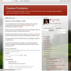
Finally, it seems, it is not incredibly clunky to write math in Blogger. In fact, it is as convenient as writing it in a native LaTeX document. The latest avataar of MathJax, while not really new, is new to me. Here are a few links which describe how to go about empowering your Blogger account. The easiest permanent fix is to add some script in your Blogger template file, as described here. Stats.norm — SciPy v0.11 Reference Guide. Stats.poisson — SciPy v0.11 Reference Guide. A Poisson discrete random variable.
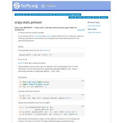
As an instance of the rv_discrete class, poisson object inherits from it a collection of generic methods (see below for the full list), and completes them with details specific for this particular distribution. Notes The probability mass function for poisson is: Distributions in SciPy. This page summarizes how to work with univariate probability distributions using Python's SciPy library.
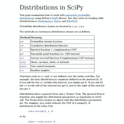
See also notes on working with distributions in Mathematica , Excel , and R/S-PLUS . Probability distribution classes are located in scipy.stats . The methods on continuous distribution classes are as follows. Functions such as pdf and cdf are defined over the entire real line. For example, the beta distribution is commonly defined on the interval [0, 1]. Finite Difference Method. Finite Difference Method using MATLAB This section considers transient heat transfer and converts the partial differential equation to a set of ordinary differential equations, which are solved in MATLAB.
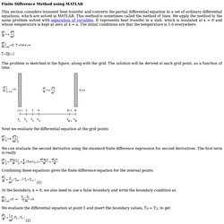
This method is sometimes called the method of lines. We apply the method to the same problem solved with separation of variables. Finite difference method. In mathematics, finite-difference methods (FDM) are numerical methods for approximating the solutions to differential equations using finite difference equations to approximate derivatives.
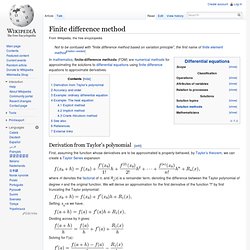
Derivation from Taylor's polynomial[edit] First, assuming the function whose derivatives are to be approximated is properly-behaved, by Taylor's theorem, we can create a Taylor Series expansion where n! Denotes the factorial of n, and Rn(x) is a remainder term, denoting the difference between the Taylor polynomial of degree n and the original function. We will derive an approximation for the first derivative of the function "f" by first truncating the Taylor polynomial:
Engineering With Python. Simple statistics with SciPy. Scipy, and Numpy, provide a host of functions for performing statistical calculations. This article will describe ways of performing a few simple statistical calculations, as an introduction to using Scipy. Scipy package is organized into several sub-packages. Before using any of these sub-packages, it must be explicitly imported. SciPy Tutorial. Travis E.
Oliphant October 21, 2004 1 Introduction SciPy is a collection of mathematical algorithms and convenience functions built on the Numeric extension for Python. It adds significant power to the interactive Python session by exposing the user to high-level commands and classes for the manipulation and visualization of data. The additional power of using SciPy within Python, however, is that a powerful programming language is also available for use in developing sophisticated programs and specialized applications. Optimization and root finding (scipy.optimize) — SciPy v0.11.dev Reference Guide.
Optimize.brute — SciPy v0.11.dev Reference Guide. Minimize a function over a given range by brute force.
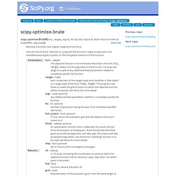
Uses the “brute force” method, i.e. computes the function’s value at each point of a multidimensional grid of points, to find the global minimum of the function. See also anneal Another approach to seeking the global minimum of multivariate, multimodal Notes Note 1: The program finds the gridpoint at which the lowest value of the objective function occurs. Module SciPy.optimize.optimize. Calculating and plotting confidence bands for linear regression models. Optimization (scipy.optimize) — SciPy v0.11.dev Reference Guide. The scipy.optimize package provides several commonly used optimization algorithms. A detailed listing is available: scipy.optimize (can also be found by help(scipy.optimize)). Below, several examples demonstrate their basic usage. Unconstrained minimization of multivariate scalar functions (minimize) The minimize function provides a common interface to unconstrained and constrained minimization algorithms for multivariate scalar functions in scipy.optimize. To demonstrate the minimization function consider the problem of minimizing the Rosenbrock function of variables:
Ubuntu Start Page. MathJax TeX and LaTeX Support — MathJax v2.0 documentation. The support for TeX and LaTeX in MathJax consists of two parts: the tex2jax preprocessor, and the TeX input processor. The first of these looks for mathematics within your web page (indicated by math delimiters like $$...$$) and marks the mathematics for later processing by MathJax.
The TeX input processor is what converts the TeX notation into MathJax’s internal format, where one of MathJax’s output processors then displays it in the web page. The tex2jax preprocessor can be configured to look for whatever markers you want to use for your math delimiters. See the tex2jax configuration options section for details on how to customize the action of tex2jax.
The TeX input processor handles conversion of your mathematical notation into MathJax’s internal format (which is essentially MathML), and so acts as a TeX to MathML converter. Note that the TeX input processor implements only the math-mode macros of TeX and LaTeX, not the text-mode macros. TeX and LaTeX in HTML documents Action AMScd. Basic model of virus infection — python v0.1 documentation. Import numpy from scipy import integrate import pylab # x = y[0] = uninfected cells # y = y[1] = infected cells # v = y[2] = virus def f ( y , t , gamma , d , a , beta , k , u ): return ( gamma - d * y [ 0 ] - beta * y [ 0 ] * y [ 2 ], beta * y [ 0 ] * y [ 2 ] - a * y [ 1 ], k * y [ 1 ] - u * y [ 2 ]) if __name__ == '__main__' : y0 = [ 1e5 , 0 , 1 ] t = numpy . arange ( 0 , 50 , 0.1 ) gamma = 1e5 d = 0.1 a = 0.5 beta = 2e-7 k = 100 u = 5 r = integrate . odeint ( f , y0 , t , args = ( gamma , d , a , beta , k , u )) pylab . plot ( t , r , '-' ) pylab . legend ([ 'Uninfected' , 'Infected' , 'Virus' ], loc = 'upper right' ) pylab . xlabel ( 'Time' ) pylab . ylabel ( 'Concentration' ) pylab . title ( 'Basic viral model' ) pylab . show ()
Latin Hypercube Sampling « Mathieu Fenniak's Weblog. Introduction Latin hypercube sampling (LHS) is a form of stratified sampling that can be applied to multiple variables. The method commonly used to reduce the number or runs necessary for a Monte Carlo simulation to achieve a reasonably accurate random distribution. LHS can be incorporated into an existing Monte Carlo model fairly easily, and work with variables following any analytical probability distribution.
Monte-Carlo simulations provide statistical answers to problems by performing many calculations with randomized variables, and analyzing the trends in the output data. Data fitting using fmin. We have seen already how to find the minimum of a function using fmin, in this example we will see how use it to fit a set of data with a curve minimizing an error function:
Integrating an initial value problem (single ODE) Cookbook/LoktaVolterraTutorial - This example describes how to integrate ODEs with the scipy.integrate module, and how to use the matplotlib module to plot trajectories, direction fields and other information. Multiple Matrix Multiplication in numpy « James Hensman’s Weblog. There are two ways to deal with matrices in numpy. The standard numpy array in it 2D form can do all kinds of matrixy stuff, like dot products, transposes, inverses, or factorisations, though the syntax can be a little clumsy. For those who just can’t let go of matlab, there’s a matrix object which prettifies the syntax somewhat. For example, to do Despite the nicer syntax in the matrix version, I prefer to use arrays. This is in part because they play nicer with the rest of numpy, but mostly because they behave better in higher dimensions.
Cookbook/Zombie Apocalypse ODEINT - Cookbook/CoupledSpringMassSystem - This cookbook example shows how to solve a system of differential equations. (Other examples include the Lotka-Volterra Tutorial , the Zombie Apocalypse and the KdV example .) This figure shows the system to be modeled: Genetic Diffusion Across a Geographic Barrier. ODE Solver using Euler Method. Simple Cellular Automata. How to draw commutative diagrams in LaTeX with TikZ. Popular Python recipes. Welcome, guest | Sign In | My Account | Store | Cart ActiveState Code » Recipes LanguagesTagsAuthorsSets Popular Python recipes Tags: Recipe 1 to 20 of 4591. Class SciPy.integrate.ode.ode. A Simple LateX Template. Integrate.ode — SciPy v0.11.dev Reference Guide.
Scipy - Integrate stiff ODEs with Python. TikZ examples tag: Diagrams. Home > TikZ > Examples > Tag: Diagrams Diagrams examples.