
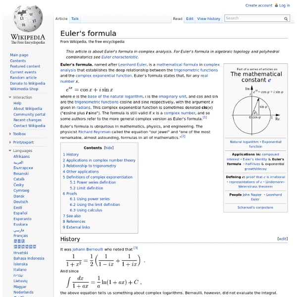
Complex plane Geometric representation of z and its conjugate z̅ in the complex plane. The distance along the light blue line from the origin to the point z is the modulus or absolute value of z. The angle φ is the argument of z. In mathematics, the complex plane or z-plane is a geometric representation of the complex numbers established by the real axis and the orthogonal imaginary axis. Notational conventions[edit] In complex analysis the complex numbers are customarily represented by the symbol z, which can be separated into its real (x) and imaginary (y) parts, like this: for example: z = 4 + 5i, where x and y are real numbers, and i is the imaginary unit. In the Cartesian plane the point (x, y) can also be represented in polar coordinates as where Here |z| is the absolute value or modulus of the complex number z; θ, the argument of z, is usually taken on the interval 0 ≤ θ < 2π; and the last equality (to |z|eiθ) is taken from Euler's formula. Stereographic projections[edit] Cutting the plane[edit]
Muḥammad ibn Mūsā al-Khwārizmī Abū ʿAbdallāh Muḥammad ibn Mūsā al-Khwārizmī[note 1][pronunciation?] (Arabic: عَبْدَالله مُحَمَّد بِن مُوسَى اَلْخْوَارِزْمِي), earlier transliterated as Algoritmi or Algaurizin, (c. 780 – c. 850) was a Persian[1][5] mathematician, astronomer and geographer during the Abbasid Empire, a scholar in the House of Wisdom in Baghdad. Some words reflect the importance of al-Khwarizmi's contributions to mathematics. "Algebra" is derived from al-jabr, one of the two operations he used to solve quadratic equations. Life He was born in a Persian[1][5] family, and his birthplace is given as Chorasmia[9] by Ibn al-Nadim. Few details of al-Khwārizmī's life are known with certainty. Al-Tabari gave his name as Muhammad ibn Musa al-Khwārizmī al-Majousi al-Katarbali (محمد بن موسى الخوارزميّ المجوسـيّ القطربّـليّ). Regarding al-Khwārizmī's religion, Toomer writes: Another epithet given to him by al-Ṭabarī, "al-Majūsī," would seem to indicate that he was an adherent of the old Zoroastrian religion. D. and J.
Complex number A complex number can be visually represented as a pair of numbers (a, b) forming a vector on a diagram called an Argand diagram, representing the complex plane. "Re" is the real axis, "Im" is the imaginary axis, and i is the imaginary unit which satisfies i2 = −1. A complex number is a number that can be expressed in the form a + bi, where a and b are real numbers and i is the imaginary unit, that satisfies the equation x2 = −1, that is, i2 = −1.[1] In this expression, a is the real part and b is the imaginary part of the complex number. Complex numbers extend the concept of the one-dimensional number line to the two-dimensional complex plane (also called Argand plane) by using the horizontal axis for the real part and the vertical axis for the imaginary part. As well as their use within mathematics, complex numbers have practical applications in many fields, including physics, chemistry, biology, economics, electrical engineering, and statistics. Overview[edit] Definition[edit] . or or z*.
Multivalued function In mathematics, a multivalued function (short form: multifunction; other names: many-valued function, set-valued function, set-valued map, multi-valued map, multimap, correspondence, carrier) is a left-total relation; that is, every input is associated with at least one output. Examples[edit] Every real number greater than zero has two square roots. The square roots of 4 are in the set {+2,−2}. The square root of 0 is 0.Each complex number except zero has two square roots, three cube roots, and in general n nth roots. As a consequence, arctan(1) is intuitively related to several values: π/4, 5π/4, −3π/4, and so on. The indefinite integral can be considered as a multivalued function. These are all examples of multivalued functions that come about from non-injective functions. Multivalued functions of a complex variable have branch points. Set-valued analysis[edit] Set-valued analysis is the study of sets in the spirit of mathematical analysis and general topology. History[edit]
Avogadro constant Previous definitions of chemical quantity involved Avogadro's number, a historical term closely related to the Avogadro constant but defined differently: Avogadro's number was initially defined by Jean Baptiste Perrin as the number of atoms in one gram-molecule of hydrogen. It was later redefined as the number of atoms in 12 grams of the isotope carbon-12 and still later generalized to relate amounts of a substance to their molecular weight.[4] For instance, to a first approximation, 1 gram of hydrogen, which has a mass number of 1 (atomic number 1), has 6.022×10²³ hydrogen atoms. Similarly, 12 grams of carbon 12, with the mass number of 12 (atomic number 6), has the same number of carbon atoms, 6.022×10²³. Avogadro's number is a dimensionless quantity and has the numerical value of the Avogadro constant given in base units. The Avogadro constant is fundamental to understanding both the makeup of molecules and their interactions and combinations. History[edit] [dubious ] Measurement[edit]
List of things named after Leonhard Euler In mathematics and physics, there are a large number of topics named in honor of Leonhard Euler, many of which include their own unique function, equation, formula, identity, number (single or sequence), or other mathematical entity. Unfortunately, many of these entities have been given simple and ambiguous names such as Euler's function, Euler's equation, and Euler's formula. Euler's work touched upon so many fields that he is often the earliest written reference on a given matter. Physicists and mathematicians sometimes jest that, in an effort to avoid naming everything after Euler, discoveries and theorems are named after the "first person after Euler to discover it".[1][2] Euler's conjectures[edit] Euler's equations[edit] Euler's formulas[edit] Euler's functions[edit] Euler's identities[edit] Euler's numbers[edit] Euler's theorems[edit] Euler's laws[edit] Other things named after Euler[edit] Topics by field of study[edit] Selected topics from above, grouped by subject. Graph theory[edit]
Imaginary unit i in the complex or cartesian plane. Real numbers lie on the horizontal axis, and imaginary numbers lie on the vertical axis There are in fact two complex square roots of −1, namely i and −i, just as there are two complex square roots of every other real number, except zero, which has one double square root. In contexts where i is ambiguous or problematic, j or the Greek ι (see alternative notations) is sometimes used. In the disciplines of electrical engineering and control systems engineering, the imaginary unit is often denoted by j instead of i, because i is commonly used to denote electric current in these disciplines. For the history of the imaginary unit, see Complex number: History. Definition[edit] With i defined this way, it follows directly from algebra that i and −i are both square roots of −1. Similarly, as with any non-zero real number: i and −i[edit] and are solutions to the matrix equation Proper use[edit] (incorrect). (ambiguous). Similarly: The calculation rules Properties[edit]
Bernoulli polynomials In mathematics, the Bernoulli polynomials occur in the study of many special functions and in particular the Riemann zeta function and the Hurwitz zeta function. This is in large part because they are an Appell sequence, i.e. a Sheffer sequence for the ordinary derivative operator. Unlike orthogonal polynomials, the Bernoulli polynomials are remarkable in that the number of crossings of the x-axis in the unit interval does not go up as the degree of the polynomials goes up. In the limit of large degree, the Bernoulli polynomials, appropriately scaled, approach the sine and cosine functions. Bernoulli polynomials Representations[edit] Explicit formula[edit] for n ≥ 0, where bk are the Bernoulli numbers. Generating functions[edit] The generating function for the Bernoulli polynomials is The generating function for the Euler polynomials is Representation by a differential operator[edit] The Bernoulli polynomials are also given by cf. integrals below. Representation by an integral operator[edit] . and
Radius of convergence Definition[edit] For a power series ƒ defined as: where cn is the nth complex coefficient, and z is a complex variable. The radius of convergence r is a nonnegative real number or ∞ such that the series converges if and diverges if In other words, the series converges if z is close enough to the center and diverges if it is too far away. Finding the radius of convergence[edit] Two cases arise. then you take certain limits and find the precise radius of convergence. Theoretical radius[edit] The radius of convergence can be found by applying the root test to the terms of the series. "lim sup" denotes the limit superior. and diverges if the distance exceeds that number; this statement is the Cauchy–Hadamard theorem. The limit involved in the ratio test is usually easier to compute, and when that limit exists, it shows that the radius of convergence is finite. This is shown as follows. That is equivalent to Practical estimation of radius[edit] Domb–Sykes plot of the function as a function of index . by
Contributions of Leonhard Euler to mathematics Mathematical notation[edit] Euler introduced much of the mathematical notation in use today, such as the notation f(x) to describe a function and the modern notation for the trigonometric functions. He was the first to use the letter e for the base of the natural logarithm, now also known as Euler's number. The use of the Greek letter to denote the ratio of a circle's circumference to its diameter was also popularized by Euler (although it did not originate with him).[1] He is also credited for inventing the notation i to denote Complex analysis[edit] A geometric interpretation of Euler's formula Euler made important contributions to complex analysis. , the complex exponential function satisfies This has been called "The most remarkable formula in mathematics " by Richard Feynman. [3] Euler's identity is a special case of this: This identity is particularly remarkable as it involves e, , i, 1, and 0, arguably the five most important constants in mathematics. Analysis[edit] for any positive real
Kepler conjecture The Kepler conjecture, named after the 17th-century German mathematician and astronomer Johannes Kepler, is a mathematical conjecture about sphere packing in three-dimensional Euclidean space. It says that no arrangement of equally sized spheres filling space has a greater average density than that of the cubic close packing (face-centered cubic) and hexagonal close packing arrangements. The density of these arrangements is slightly greater than 74%. In 1998 Thomas Hales, following an approach suggested by Fejes Tóth (1953), announced that he had a proof of the Kepler conjecture. Hales' proof is a proof by exhaustion involving the checking of many individual cases using complex computer calculations. Referees have said that they are "99% certain" of the correctness of Hales' proof, so the Kepler conjecture is now very close to being accepted as a theorem. Background[edit] Diagrams of cubic close packing (left) and hexagonal close packing (right). Origins[edit] Nineteenth century[edit]