
Borromean rings Mathematical properties[edit] Although the typical picture of the Borromean rings (above right picture) may lead one to think the link can be formed from geometrically ideal circles, they cannot be. Freedman and Skora (1987) prove that a certain class of links, including the Borromean links, cannot be exactly circular. A realization of the Borromean rings as ellipses 3D image of Borromean Rings Linking[edit] In knot theory, the Borromean rings are a simple example of a Brunnian link: although each pair of rings is unlinked, the whole link cannot be unlinked. Simplest is that the fundamental group of the complement of two unlinked circles is the free group on two generators, a and b, by the Seifert–van Kampen theorem, and then the third loop has the class of the commutator, [a, b] = aba−1b−1, as one can see from the link diagram: over one, over the next, back under the first, back under the second. Hyperbolic geometry[edit] Connection with braids[edit] History[edit] Partial rings[edit]
Tangent Tangent to a curve. The red line is tangential to the curve at the point marked by a red dot. Tangent plane to a sphere As it passes through the point where the tangent line and the curve meet, called the point of tangency, the tangent line is "going in the same direction" as the curve, and is thus the best straight-line approximation to the curve at that point. The word tangent comes from the Latin tangere, to touch. History[edit] The first definition of a tangent was "a right line which touches a curve, but which when produced, does not cut it".[1] This old definition prevents inflection points from having any tangent. Pierre de Fermat developed a general technique for determining the tangents of a curve using his method of adequality in the 1630s. Leibniz defined the tangent line as the line through a pair of infinitely close points on the curve. Tangent line to a curve[edit] At each point, the line is always tangent to the curve. Analytical approach[edit] Intuitive description[edit] by but If
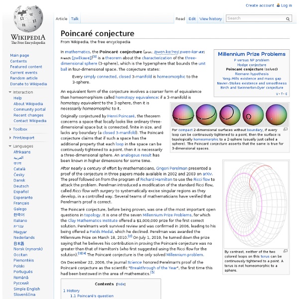
Holonomy Parallel transport on a sphere depends on the path. Transporting from A → N → B → A yields a vector different from the initial vector. This failure to return to the initial vector is measured by the holonomy of the connection. The study of Riemannian holonomy has led to a number of important developments. The holonomy was introduced by Cartan (1926) in order to study and classify symmetric spaces. It was not until much later that holonomy groups would be used to study Riemannian geometry in a more general setting. Definitions[edit] Holonomy of a connection in a vector bundle[edit] The restricted holonomy group based at x is the subgroup coming from contractible loops γ. If M is connected then the holonomy group depends on the basepoint x only up to conjugation in GL(k, R). Choosing different identifications of Ex with Rk also gives conjugate subgroups. Some important properties of the holonomy group include: Holonomy of a connection in a principal bundle[edit] such that . In particular,
Sine For the angle α, the sine function gives the ratio of the length of the opposite side to the length of the hypotenuse. The sine function graphed on the Cartesian plane. In this graph, the angle x is given in radians (π = 180°). The sine and cosine functions are related in multiple ways. The derivative of is . . In mathematics, the sine function is a trigonometric function of an angle. The sine function is commonly used to model periodic phenomena such as sound and light waves, the position and velocity of harmonic oscillators, sunlight intensity and day length, and average temperature variations throughout the year. The function sine can be traced to the jyā and koṭi-jyā functions used in Gupta period Indian astronomy (Aryabhatiya, Surya Siddhanta), via translation from Sanskrit to Arabic and then from Arabic to Latin.[1] The word "sine" comes from a Latin mistranslation of the Arabic jiba, which is a transliteration of the Sanskrit word for half the chord, jya-ardha.[2] Identities[edit] and
Riemannian manifold In differential geometry, a (smooth) Riemannian manifold or (smooth) Riemannian space (M,g) is a real smooth manifold M equipped with an inner product on the tangent space at each point that varies smoothly from point to point in the sense that if X and Y are vector fields on M, then is a smooth function. The family of inner products is called a Riemannian metric (tensor). A Riemannian metric (tensor) makes it possible to define various geometric notions on a Riemannian manifold, such as angles, lengths of curves, areas (or volumes), curvature, gradients of functions and divergence of vector fields. Introduction[edit] In 1828, Carl Friedrich Gauss proved his Theorema Egregium (remarkable theorem in Latin), establishing an important property of surfaces. Overview[edit] Smoothness of α(t) for t in [0, 1] guarantees that the integral L(α) exists and the length of this curve is defined. Riemannian manifolds as metric spaces[edit] Properties[edit] Riemannian metrics[edit] Examples[edit] Isometries[edit]
Cosine The cosine function is one of the basic functions encountered in trigonometry (the others being the cosecant, cotangent, secant, sine, and tangent). Let be an angle measured counterclockwise from the x-axis along the arc of the unit circle. is the horizontal coordinate of the arc endpoint. The common schoolbook definition of the cosine of an angle in a right triangle (which is equivalent to the definition just given) is as the ratio of the lengths of the side of the triangle adjacent to the angle and the hypotenuse, i.e., A convenient mnemonic for remembering the definition of the sine, cosine, and tangent is SOHCAHTOA (sine equals opposite over hypotenuse, cosine equals adjacent over hypotenuse, tangent equals opposite over adjacent). As a result of its definition, the cosine function is periodic with period . also obeys the identity The definition of the cosine function can be extended to complex arguments using the definition The cosine function has a fixed point at 0.739085... for is where via
Ricci flow Several stages of Ricci flow on a 2D manifold. In differential geometry, the Ricci flow (/ˈriːtʃi/) is an intrinsic geometric flow. It is a process that deforms the metric of a Riemannian manifold in a way formally analogous to the diffusion of heat, smoothing out irregularities in the metric. Mathematical definition[edit] Given a Riemannian manifold with metric tensor , we can compute the Ricci tensor The normalized Ricci flow makes sense for compact manifolds and is given by the equation where is the average (mean) of the scalar curvature (which is obtained from the Ricci tensor by taking the trace) and is the dimension of the manifold. The factor of −2 is of little significance, since it can be changed to any nonzero real number by rescaling t. Informally, the Ricci flow tends to expand negatively curved regions of the manifold, and contract positively curved regions. Examples[edit] If the manifold is Euclidean space, or more generally Ricci-flat, then Ricci flow leaves the metric unchanged.
Cardioid A cardioid generated by a rolling circle around another circle and tracing one point on the edge of it. A cardioid given as the envelope of circles whose centers lie on a given circle and which pass through a fixed point on the given circle. The name was coined by de Castillon in 1741[2] but had been the subject of study decades beforehand.[3] Named for its heart-like form, it is shaped more like the outline of the cross section of a round apple without the stalk. A cardioid microphone exhibits an acoustic pickup pattern that, when graphed in two dimensions, resembles a cardioid, (any 2d plane containing the 3d straight line of the microphone body.) Equations[edit] Based on the rolling circle description, with the fixed circle having the origin as its center, and both circles having radius a, the cardioid is given by the following parametric equations: In the complex plane this becomes or, in rectangular coordinates, or, in the complex plane, With the substitution u=tan t/2, or . is a cardioid.
Hadamard space In an Hadamard space, a triangle is hyperbolic; that is, the middle one in the picture. In fact, any complete metric space where a triangle is hyperbolic is an Hadamard space. In geometry, an Hadamard space, named after Jacques Hadamard, is a non-linear generalization of a Hilbert space. It is defined to be a nonempty[1] complete metric space where, given any points x, y, there exists a point m such that for every point z, The point m is then the midpoint of x and y: In a Hilbert space, the above inequality is equality (with ), and in general an Hadamard space is said to be flat if the above inequality is equality. fixes the circumcenter of B. The basic result for a non-positively curved manifold is the Cartan–Hadamard theorem. See also[edit] References[edit] Jump up ^ The assumption on "nonempty" has meaning: a fixed point theorem often states the set of fixed point is an Hadamard space.