Lecture schedule. Lecture Schedule The lectures are all taped, and have been posted on Tech TV and are linked below..
Lecture schedule Lecture 1 (Th 9/5) (Postscript, PDF, video) Definitions of computational neuroscience and neural networks. Classical neural network equations. Learning rule. Learning rule or Learning process is a method or a mathematical logic which improves the neural network's performance and usually this rule is applied repeatedly over the network.
It is done by updating the weights and bias levels of a network when a network is simulated in a specific data environment.[1] A learning rule may accept existing condition ( weights and bias ) of the network and will compare the expected result and actual result of the network to give new and improved values for weights and bias. [2] Depending on the complexity of actual model, which is being simulated, the learning rule of the network can be as simple as an XOR gate or Mean Squared Error or it can be the result of multiple differential equations.
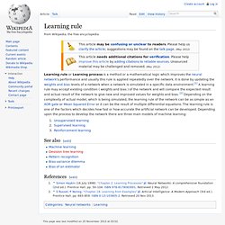
The learning rule is one of the factors which decides how fast or how accurate the artificial network can be developed. Depending upon the process to develop the network there are three main models of machine learning: See also[edit] References[edit] Perceptron learning algorithm. The perceptron learning rule was originally developed by Frank Rosenblatt in the late 1950s.
Training patterns are presented to the network's inputs; the output is computed. Then the connection weights wjare modified by an amount that is proportional to the product of the difference between the actual output, y, and the desired output, d, and the input pattern, x. The algorithm is as follows: Initialize the weights and threshold to small random numbers. Present a vector x to the neuron inputs and calculate the output. Update the weights according to: where d is the desired output, t is the iteration number, and eta is the gain or step size, where 0.0 < n < 1.0 Repeat steps 2 and 3 until: the iteration error is less than a user-specified error threshold or a predetermined number of iterations have been completed. Hebb's Learning. Next: Hopfield Network Up: Introduction to Neural Networks Previous: Paradigms of Learning Donald Hebb (Canadian Psychologist) speculated in 1949 that ``When neuron A repeatedly and persistently takes part in exciting neuron B, the synaptic connection from A to B will be strengthened.'' Simultaneous activation of neurons leads to pronounced increases in synaptic strength between them.
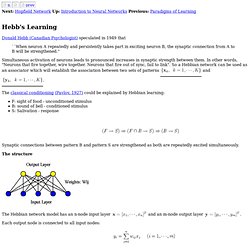
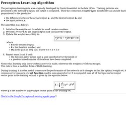
In other words, "Neurons that fire together, wire together. Neurons that fire out of sync, fail to link". Widrow-Hoff Learning LMS. Backpropagation. The project describes teaching process of multi-layer neural network employing backpropagation algorithm.
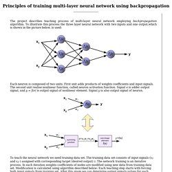
To illustrate this process the three layer neural network with two inputs and one output,which is shown in the picture below, is used: Each neuron is composed of two units. First unit adds products of weights coefficients and input signals. The second unit realise nonlinear function, called neuron activation function. Signal e is adder output signal, and y = f(e) is output signal of nonlinear element.
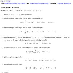
Learning representations by back-propagating errors. BPTT. Summary of BP training. Next: Radial-Basis Function (RBF) Networks Up: Back Propagation Network (BPN) Previous: Error back propagation Summary of BP training The following is for one randomly chosen training pattern pair Apply to the input nodes; Compute net input to and output from all nodes in the hidden layer: Compute net input to and output from all nodes in the output layer: Compare the output with the desired output corresponding to the input , to find the error terms for all output nodes (not quite the same as defined previously): Find error terms for all hidden nodes (not quite the same as defined previously) Update weights to output nodes Update weights to hidden nodes Compute This process is then repeated with another pair of.
Neuron Model and Network Architectures (Neural Network Toolbox) Batch Training Batch training, in which weights and biases are only updated after all of the inputs and targets are presented, can be applied to both static and dynamic networks.
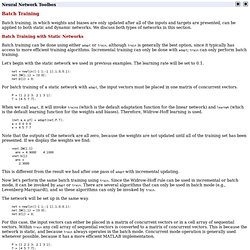
We discuss both types of networks in this section. Competitive Learning. Next: Self-Organizing Map (SOM) Up: Competitive Learning Networks Previous: Competitive Learning Networks Competitive Learning Competitive learning is a typical unsupervised learning network, similar to the statistical clustering analysis methods (k-means, Isodata).
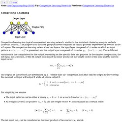
The purpose is to discover groups/clusters composed of similar patterns represented by vectors in the n-D space. Learning Vector Quantization (LVQ) Self-Organizing Map (SOM) Next: Self-organizing property of the Up: Competitive Learning Networks Previous: Competitive Learning Self-Organizing Map (SOM) Self-organizing map (SOM), also referred to as self-organized feature mapping (SOFM), is a process that maps the input patterns in a high-dimensional vector space to a low-dimensional (typically 2-D) output space, the feature map, so that the nodes in the neighborhood of this map respond similarly to a group of similar input patterns.
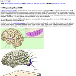
The idea of SOM is motivated by the mapping process in the brain, by which signals from various sensory (e.g., visual and auditory) system are projected (mapped) to different 2-D cortical areas and responded to by the neurons wherein. For example, sound signals of different frequencies are mapped to the primary auditory cortex in which neighboring neurons respond to similar frequencies. , but also at a set of output nodes. Autoassociative memory. Autoassociative memory, also known as auto-association memory or an autoassociation network, is often misunderstood to be only a form of backpropagation or other neural networks.
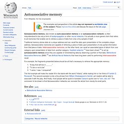
It is actually a more generic term that refers to all memories that enable one to retrieve a piece of data from only a tiny sample of itself. Traditional memory stores data at a unique address and can recall the data upon presentation of the complete unique address. Autoassociative memories are capable of retrieving a piece of data upon presentation of only partial information from that piece of data. Heteroassociative memories, on the other hand, can recall an associated piece of datum from one category upon presentation of data from another category.
Hopfield networks [1] have been shown [2] to act as autoassociative memory since they are capable of remembering data by observing a portion of that data. "A day that will live in ______""To be or not to be""I came, I saw, I conquered" See also[edit] Hopfield Neural Network. Hopfield Network Simulation Hopfield Network is an example of the network with feedback (so-called recurrent network), where outputs of neurons are connected to input of every neuron by means of the appropriate weights. Of course there are also inputs which provide neurons with components of test vector. A Binary Hopfield Neural Network Applet. Introduction The Hopfield model is a distributed model of an associative memory. Neurons are pixels and can take the values of -1 (off) or +1 (on). The network has stored a certain number of pixel patterns. Hopfield Network. Next: Perceptron Learning Up: Introduction to Neural Networks Previous: Hebb's Learning Hopfield network(Hopfield 1982) is recurrent network composed of a set of nodes and behaves as an auto-associator (content addressable memory) with a set of patterns stored in it.
The network is first trained in the fashion similar to that of the Hebbian learning, and then used as an auto-associator. Presented with a new input pattern (e.g., noisy, incomplete version of some pre-stored pattern) BAM. Simple Recurrent Network. Since the publication of the original pdp books (Rumelhart et al., 1986; McClelland et al., 1986) and back-propagation algorithm, the bp framework has been developed extensively. Two of the extensions that have attracted the most attention among those interested in modeling cognition have been the Simple Recurrent Network (SRN) and the recurrent back-propagation (RBP) network. In this and the next chapter, we consider the cognitive science and cognitive neuroscience issues that have motivated each of these models, and discuss how to run them within the PDPTool framework. 7.1.1 The Simple Recurrent Network The Simple Recurrent Network (SRN) was conceived and first used by Jeff Elman, and was first published in a paper entitled Finding structure in time (Elman, 1990).
Figure 7.1: The SRN network architecture. An SRN of the kind Elman employed is illustrated in Figure 7.1. Elman Neural Network SRN.