
Extracting JPEG DCT coefficients. DCT / IDCT Example utilisé. Standard JPEG compression uses (1) 8x8 Discrete Cosine Transform, (2) quantization based on certain luminance + chrominance tables, and (3) entropy-encoding (Huffman coding).
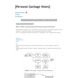
Here, I'm using OpenCV (Python) to simulate DCT + quantization + IDCT, without Huffman coding. jpeg.orgwikipedia/jpegopencv Ref: "Image and Video Compression for Multimedia Engineering", Yun Q.Shi, Huifang Sun, CRC Press, 2000. "Digital Image Processing", Third Ed., Rafael C. Gonzalez, Richard E. (Image courtesy of Yun Q.Shi, Huifang Sun, CRC Press, taken from the book referenced above.)
Jpeg: Colorspace Transform, Subsampling, DCT and Quantisation — Multimedia Codec Excercises 1.0 documentation. In this document the first 4 steps of the JPEG encoding chain are demonstrated.

These 4 steps contain the lossy parts of the coding. The remaining steps, i.e. runlength and Huffman encoding, are losless. Therefore the 4 steps demonstrated here are sufficient to study the quality-loss of JPEG encoding. The following packages are required. IDCT frequencies. There is a DFT sample in the OpenCV samples folder (see dft.cpp), but unfortunately no DCT sample :( The reference docu about OpenCV's dct() function tells you how to call the method, but there are no details how to prepare the input image matrix :( Here is an important note about the matrix type needed for the dct() function (CV_64F) which helped me a lot.

It took me an hour, but now I figured out how to do the DCT using OpenCV. There are two important points: image dimensions have to be a multiple of 2 image input matrix that goes into dct() has to be of type float Here is the code: The original image will be transformed to a frequency matrix which looks visualized using gray-values like this: When we iteratively take more and more higher frequencies as input for the idct() function, we can see how we can see more and more details: These images were generated with the above code which should show you how to use OpenCV's dct() function. So let's save only these 100×100 low frequencies. Transformations — Multimedia Codec Excercises 1.0 documentation. This section demonstrates the Discrete Cosine Transform of an image.
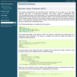
As in the Jpeg standard the DCT is performed blockwise. The entire image is partitioned into non-overlapping blocks of size (8x8) pixels. The transformed image is backtransformed by applying the Inverse Discrete Cosine Transform (IDCT). The reconstructed image is identical to the original image. Moreover, this Python program allows the user to select an arbitrary block in the image (by clicking into the image). The following packages are applied by this program import cv2import numpy as npfrom matplotlib import pyplot as pltfrom matplotlib.colors import Normalizeimport matplotlib.cm as cm The height and width of the blocks is B=8.
B=8 #blocksizefn3= 'tria.jpg'img1 = cv2.imread(fn3, cv2.CV_LOAD_IMAGE_GRAYSCALE)h,w=np.array(img1.shape[:2])/B * Bprint hprint wimg1=img1[:h,:w] Discrete Cosine Transform and A Case Study on Image Compression. The Discrete Cosine Transform (DCT) Next: Differential Encoding Up: Source Coding Techniques Previous: Relationship between DCT and The discrete cosine transform (DCT) helps separate the image into parts (or spectral sub-bands) of differing importance (with respect to the image's visual quality).
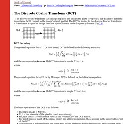
The DCT is similar to the discrete Fourier transform: it transforms a signal or image from the spatial domain to the frequency domain (Fig 7.8). Transformée en cosinus discrète. Un article de Wikipédia, l'encyclopédie libre.
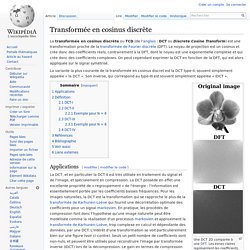
La transformée en cosinus discrète ou TCD (de l'anglais : DCT ou Discrete Cosine Transform) est une transformation proche de la transformée de Fourier discrète (DFT). Le noyau de projection est un cosinus et crée donc des coefficients réels, contrairement à la DFT, dont le noyau est une exponentielle complexe et qui crée donc des coefficients complexes. On peut cependant exprimer la DCT en fonction de la DFT, qui est alors appliquée sur le signal symétrisé.
La variante la plus courante de la transformée en cosinus discret est la DCT type-II, souvent simplement appelée « la DCT ». Son inverse, qui correspond au type-III est souvent simplement appelée « IDCT ». Une DCT 2D comparée à une DFT. Applications[modifier | modifier le code] Lecture_5. CSE 228 Week 3 Part 1 JPEG Stages There are many transforms, most of which are very slow.

This is important to consider since video demands real-time encoding and decoding. The JPEG committee took suggestions and empirically studied the use of several different transforms. Of the transforms studied, DCT (Discrete Cosine Transform) proved superior. In JPEG, DCT operates on one block at a time. Formula for FDCT: Notes about DCT: The results of a 64-element DCT transform are 1 DC coefficient and 63 AC coefficients. Zig-Zag sequencing: Note that each diagonal line in this zig-zag sequence contains AC coefficients whose sum is constant. Why is this ordering important? The 8x8 region of pixels highlighted above looks like this (magnified 1600 times) As you can see, this region does not deviate much from its average color.
Logically, if these values are of little importance we should be able to assign fewer bits to them in order to achieve greater compression.