
The Commons Math User Guide - Linear Algebra. 3.1 Overview Linear algebra support in commons-math provides operations on real matrices (both dense and sparse matrices are supported) and vectors.
It features basic operations (addition, subtraction ...) and decomposition algorithms that can be used to solve linear systems either in exact sense and in least squares sense. 3.2 Real matrices The RealMatrix interface represents a matrix with real numbers as entries. The following basic matrix operations are supported: Matrix addition, subtraction, multiplication Scalar addition and multiplication transpose Norm and Trace Operation on a vector Example: The three main implementations of the interface are Array2DRowRealMatrix and BlockRealMatrix for dense matrices (the second one being more suited to dimensions above 50 or 100) and SparseRealMatrix for sparse matrices. 3.3 Real vectors The RealVector interface represents a vector with real numbers as entries. 3.4 Solving linear systems For example, to solve the linear system. Non-linear least squares.
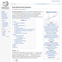
Theory[edit] Consider a set of data points, and a curve (model function) that in addition to the variable also depends on parameters, with It is desired to find the vector of parameters such that the curve fits best the given data in the least squares sense, that is, the sum of squares is minimized, where the residuals (errors) ri are given by for The minimum value of S occurs when the gradient is zero.
In a non-linear system, the derivatives are functions of both the independent variable and the parameters, so these gradient equations do not have a closed solution. Here, k is an iteration number and the vector of increments, is known as the shift vector. The Jacobian, J, is a function of constants, the independent variable and the parameters, so it changes from one iteration to the next. And the residuals are given by Substituting these expressions into the gradient equations, they become which, on rearrangement, become n simultaneous linear equations, the normal equations is positive definite). Matrix exponential. In mathematics, the matrix exponential is a matrix function on square matrices analogous to the ordinary exponential function.
Abstractly, the matrix exponential gives the connection between a matrix Lie algebra and the corresponding Lie group. The above series always converges, so the exponential of X is well-defined. Note that if X is a 1×1 matrix the matrix exponential of X is a 1×1 matrix whose single element is the ordinary exponential of the single element of X. Properties[edit] Let X and Y be n×n complex matrices and let a and b be arbitrary complex numbers. e0 = IeaXebX = e(a + b)XeXe−X = IIf XY = YX then eXeY = eYeX = e(X + Y).If Y is invertible then eYXY−1 =YeXY−1.exp(XT) = (exp X)T, where XT denotes the transpose of X. Linear differential equation systems[edit] One of the reasons for the importance of the matrix exponential is that it can be used to solve systems of linear ordinary differential equations.
Magnus expansion. In mathematics and physics, the Magnus expansion, named after Wilhelm Magnus (1907–1990), provides an exponential representation of the solution of a first order homogeneous linear differential equation for a linear operator.
In particular it furnishes the fundamental matrix of a system of linear ordinary differential equations of order n with varying coefficients. The exponent is built up as an infinite series whose terms involve multiple integrals and nested commutators. Magnus approach and its interpretation[edit] Given the n × n coefficient matrix A(t), one wishes to solve the initial value problem associated with the linear ordinary differential equation for the unknown n-dimensional vector function Y(t).
When n = 1, the solution simply reads This is still valid for n > 1 if the matrix A(t) satisfies A(t1) A(t2) = A(t2) A(t1) for any pair of values of t, t1 and t2. Where, for simplicity, it is customary to write Ω(t) for Ω(t,t0) and to take t0 = 0. Convergence of the expansion[edit] W.