
Visual Representation of SQL Joins. Introduction This is just a simple article visually explaining SQL JOINs.
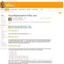
Background I'm a pretty visual person. Things seem to make more sense as a picture. I looked all over the Internet for a good graphical representation of SQL JOINs, but I couldn't find any to my liking. Using the code I am going to discuss seven different ways you can return data from two relational tables. For the sake of this article, I'll refer to 5, 6, and 7 as LEFT EXCLUDING JOIN, RIGHT EXCLUDING JOIN, and OUTER EXCLUDING JOIN, respectively. Inner JOIN This is the simplest, most understood Join and is the most common. Hide Copy Code SELECT <select_list> FROM Table_A A INNER JOIN Table_B B ON A.Key = B.Key Left JOIN This query will return all of the records in the left table (table A) regardless if any of those records have a match in the right table (table B).
SELECT <select_list>FROM Table_A A LEFT JOIN Table_B B ON A.Key = B.Key Right JOIN SELECT <select_list>FROM Table_A A RIGHT JOIN Table_B B ON A.Key = B.Key. Assessing Linear Models in R. In this post I will look at several techniques for assessing linear models in R, via the IPython Notebook interface.
I find the notebook interface to be more convenient for development and debugging because it allows one to evaluate cells instead of going back and forth between a script and a terminal. If you do not have the IPython Notebook, then you can check it out here. It is a very nice Mathematica-inspired “notebook” interface that allows you to work on bits of code in independent cells. It’s a dream come true for exploratory data analysis. If you do not already have it, you will also need to install the rpy2 module. Once all of that is squared away, you should be able to open an IPython notebook from the terminal using, and load the rmagic extension using, We will be using the rock data set that comes with R. In the rock data set, twelve core samples were sampled by four cross-sections, making a total of 48 samples. That minimizes the function, Here, Residuals. Welcome to TheFourierTransform.com - The Fourier Transform Website.
Concepts for Fourier Transforms. A signal can be viewed from two different standpoints: The frequency domain The time domain In astronomy the frequency domain is perhaps the most familiar, because a spectrometer, e.g. a prism or a diffraction grating, splits light into its component color or frequencies and permits us to record its spectral content.
This is like the trace on a spectrum analyzer, where the horizontal deflection is the frequency variable and the vertical deflection is the signals amplitude at that frequency. In the lab we are also familiar with the time domain. This is like the trace on an oscilloscope where the vertical deflection is the signals amplitude, and the horizontal deflection is the time variable. Any signal can be fully described in either of these domains.
Back to Contents or on to Applications.
Multiple regression. Machine Learning. How To Identify Patterns in Time Series Data: Time Series Analysis.