
Conditional formatting tricks: Sum values in Excel by cell color. When you think VBA code is your only hope, try combing built-it conditional formatting tools.
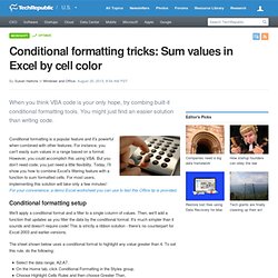
You might just find an easier solution than writing code. Conditional formatting is a popular feature and it's powerful when combined with other features. For instance, you can't easily sum values in a range based on a format. However, you could accomplish this using VBA. The Excel Magician: 70+ Excel Tips and Shortcuts to help you make Excel Magic. Posted by nitzan on Wednesday, November 28th, 2007 Are you working with Excel and want take your Excel skills to the next level?

Or do you want to learn Excel and don’t know where to start? Check out these 70+ tips and shortcuts that will help you make Excel Magic. Online tutorials & videos The following online tutorials are mostly free and will teach you quite a bit about Excel. Two ways to build dynamic charts in Excel. Users will appreciate a chart that updates right before their eyes.

In Excel 2007 and 2010 it's as easy as creating a table. In earlier versions, you'll need the formula method. If you want to advance beyond your ordinary spreadsheet skills, creating dynamic charts is a good place to begin that journey. The key is to define the chart's source data as a dynamic range. By doing so, the chart will automatically reflect changes and additions to the source data. The table method First, we'll use the table feature, available in Excel 2007 and 2010-you'll be amazed at how simple it is.
Click the Insert tab.In the Tables group, click Table.Excel will display the selected range, which you can change. Any chart you build on the table will be dynamic. Select the table.Click the Insert tab.In the Charts group, choose the first 2-D column chart in the Chart dropdown. Now, update the chart by adding values for March and watch the chart update automatically. The dynamic formula method. Create a dynamic Excel chart and make your own dashboard. A dynamic chart reuses the same chart object to chart different source values.
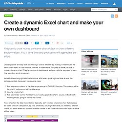
You'll save time and your users will appreciate the effort. Charting data is an easy task and reusing a chart is efficient! By reusing, I mean to use the same chart object to chart multiple sources. In other words, I'm going to show you how to create a dynamic chart. They're common in dashboards and you might be surprised to learn how easy they are to implement. Instead of launching right into the technique, let's take a quick high-end look at what this technique entails, because it has several steps: Download Build A Simple Timesheet In Excel. Make every user a power Excel user with dynamic conditional row banding. Combine data validation and conditional formatting to implement an easy-to-use dynamic banding option for your users.

Thanks to conditional formatting, you can apply several banding schemes to your Excel worksheets, and we've discussed several of them already. One possibility we haven't reviewed, however, is using data to determine which rows are banded. Throw in a little data validation and you can let users band (or shade) specific rows by simply choosing an item from a list. To illustrate this technique, we'll use data validation to display category values. When the user chooses a category, conditional formatting will shade records for the selected category. Steps Implementing this banding scheme is easier than you might think. Step One First, create a unique list of category values, as follows: Select the list of values. Step Two Now you're ready to build the validation list to make the whole process easy and intuitive for the user: Step Three Select the data range. Using it! Also read: How to find duplicates in Excel.
You'll need more than one trick up your sleeve to find duplicates in Excel.

In the duplicate world, definition means everything. That's because a duplicate is subjective to the context of its related data. Duplicates can occur within a single column, across multiple columns, or complete records. There's no one feature or technique that will find duplicates in every case. To find duplicate records, use Excel's easy-to-use Filter feature as follows: Select any cell inside the recordset.From the Data menu, choose Filter and then select Advanced Filter to open the Advanced Filter dialog box.Select Copy To Another Location in the Action section.Enter a copy range in the Copy To control.Check Unique Records Only and click OK.