
Graph traversal. Redundancy[edit] Unlike tree traversal, graph traversal may require that some nodes be visited more than once, since it is not necessarily known before transitioning to a node that it has already been explored.
As graphs become more dense, this redundancy becomes more prevalent, causing computation time to increase; as graphs become more sparse, the opposite holds true. Thus, it is usually necessary to remember which nodes have already been explored by the algorithm, so that nodes are revisited as infrequently as possible (or in the worst case, to prevent the traversal from continuing indefinitely).
This may be accomplished by associating each node of the graph with a "color" or "visitation" state during the traversal, which is then checked and updated as the algorithm visits each node. If the node has already been visited, it is ignored and the path is pursued no further; otherwise, the algorithm checks/updates the node and continues down its current path. Depth-first search. A version of depth-first search was investigated in the 19th century by French mathematician Charles Pierre Trémaux[1] as a strategy for solving mazes.[2][3] Properties[edit] The time and space analysis of DFS differs according to its application area.
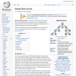
In theoretical computer science, DFS is typically used to traverse an entire graph, and takes time , linear in the size of the graph. In these applications it also uses space in the worst case to store the stack of vertices on the current search path as well as the set of already-visited vertices. For applications of DFS in relation to specific domains, such as searching for solutions in artificial intelligence or web-crawling, the graph to be traversed is often either too large to visit in its entirety or infinite (DFS may suffer from non-termination). Example[edit] For the following graph: Iterative deepening is one technique to avoid this infinite loop and would reach all nodes. Output of a depth-first search[edit] Depth First and Breadth First Search: Page 4. By kirupa | 13 January 2006 From the previous page (and prior pages), you learned how to solve search problems by hand.
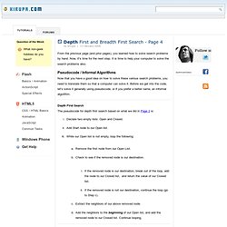
Now, it's time for the next step. It is time to help your computer to solve the search problems also. Pseudocode / Informal Algorithms Now that you have a good idea on how to solve these various search problems, you need to translate them so that a computer can solve it. Before we get into the code, let's solve it generally using pseudocode, or if you prefer a better name, an informal algorithm. Depth First Search The pseudocode for depth first search based on what we did in Page 2 is: Declare two empty lists: Open and Closed.
Breadth First Search The pseudocode for breadth first first search is similar to what you see above, and it is based on what we did in page 3 is: Declare two empty lists: Open and Closed. The Pseudocode Converted to Flash Syntax The following is Depth First search in ActionScript using methods from the Graph ADT: searchMethod = function () { Breadth-first search. In graph theory, breadth-first search (BFS) is a strategy for searching in a graph when search is limited to essentially two operations: (a) visit and inspect a node of a graph; (b) gain access to visit the nodes that neighbor the currently visited node.
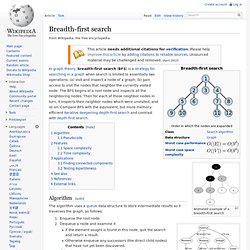
The BFS begins at a root node and inspects all the neighboring nodes. Then for each of those neighbor nodes in turn, it inspects their neighbor nodes which were unvisited, and so on. Compare BFS with the equivalent, but more memory-efficient Iterative deepening depth-first search and contrast with depth-first search. Animated example of a breadth-first search Algorithm[edit] An example map of Germany with some connections between cities The breadth-first tree obtained when running BFS on the given map and starting in Frankfurt Pseudocode[edit] Input: A graph G and a root v of G Features[edit] Space complexity[edit] where is the cardinality of the set of vertices.
. [1] space in memory, while an Adjacency matrix representation occupies and.