
CS231n Convolutional Neural Networks for Visual Recognition. Table of Contents: Convolutional Neural Networks are very similar to ordinary Neural Networks from the previous chapter: they are made up of neurons that have learnable weights and biases.
Each neuron receives some inputs, performs a dot product and optionally follows it with a non-linearity. The whole network still expresses a single differentiable score function: from the raw image pixels on one end to class scores at the other. And they still have a loss function (e.g. SVM/Softmax) on the last (fully-connected) layer and all the tips/tricks we developed for learning regular Neural Networks still apply.
So what changes? Architecture Overview Recall: Regular Neural Nets. Regular Neural Nets don’t scale well to full images. 3D volumes of neurons. Left: A regular 3-layer Neural Network. A ConvNet is made up of Layers. Layers used to build ConvNets Example Architecture: Overview. In summary: The activations of an example ConvNet architecture. Convolutional Layer The brain view. Perspective rectification – Mikko's Project Corner. This is a cool perspective rectification method that I learnt last week.
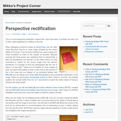
It probably has also a lot of other useful applications in addition to this one. Figure 1. For this method, you will need MATLAB and Corke’s Machine Vision Toolbox (MVTB). I needed also the MATLAB Functions for Multiple View Geometry even though I didn’t notice it in MVTB’s installation instructions but I may have failed to install the toolbox correctly. When you are ready, run the following script in MATLAB.
Figure 2. im = imread('input.jpg'); image(im); P = ginput(4)'; X = [min(P(1,:)), min(P(2,:)); max(P(1,:)), min(P(2,:)); max(P(1,:)), max(P(2,:)); min(P(1,:)), max(P(2,:))]'; H = homography(P, X); output = homwarp(H, im); imwrite(output, 'output.jpg'); The most relevant things in these lines are the homography and homwarp functions that came with MVTB. Figure 3. Now it should be easy to crop the image and do the possibly necessary width/height scaling using your favourite image editing program. Peter's Functions for Computer Vision.
Perceptually Uniform Colour Maps Many widely used colour maps have perceptual flat spots that can hide features as large as 10% of your total data range.
MATLAB's 'hot' and 'hsv' colour maps suffer from this problem. Use these colour maps instead. For an overview of this work and the theory behind it please visit this page Generation and correction of colour maps cmap.m Colour map generating function. Rendering of images with colour maps applycolourmap.m Applies a colour map to a single channel image to obtain an RGB result. showdivim.m This function is intended for displaying an image with a diverging colour map.
Test images sineramp.m Generates a test image consisting of a sine wave superimposed on a ramp function The amplitude of the sine wave is modulated from its full value at the top of the image to 0 at the bottom. Visualization of colour map paths and colour spaces.
Chapter 02. Image formation. Chapter 03. Image processing. Chapter 04. Feature extraction and matching. Chapter 05. Motion detection and tracking. Project. Software. Full courses & Books.