
Matrices. Algebra Word Problem: Distance, Rate, and Time. Solving Ratio Proportion Problems the EASY Way. Math. Fibonacci sacred geometry. Math. Wau: The Most Amazing, Ancient, and Singular Number. No, really, pi is wrong: The Tau Manifesto by Michael Hartl. Math. Nonlinear system. Typically, the behavior of a nonlinear system is described by a nonlinear system of equations.
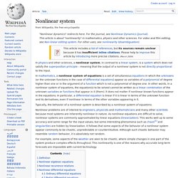
Nonlinear problems are of interest to engineers, physicists and mathematicians and many other scientists because most systems are inherently nonlinear in nature. As nonlinear equations are difficult to solve, nonlinear systems are commonly approximated by linear equations (linearization). This works well up to some accuracy and some range for the input values, but some interesting phenomena such as chaos[1] and singularities are hidden by linearization.
It follows that some aspects of the behavior of a nonlinear system appear commonly to be chaotic, unpredictable or counterintuitive. Although such chaotic behavior may resemble random behavior, it is absolutely not random. Play on the Nash: Diversity/Complexity/Threshold/Equillibrium.
Methods in math. Organisms math. Math theory. Numberphile - Videos about Numbers and Stuff. Diameter. Des maths partout ! (Fibonacci, nombre d'or, fractales & co) Right Angled Triangles. Gradient. In the above two images, the values of the function are represented in black and white, black representing higher values, and its corresponding gradient is represented by blue arrows.
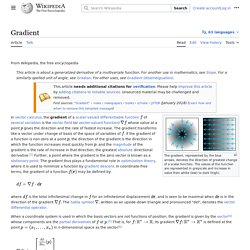
The Jacobian is the generalization of the gradient for vector-valued functions of several variables and differentiable maps between Euclidean spaces or, more generally, manifolds. A further generalization for a function between Banach spaces is the Fréchet derivative. Motivation[edit] Investigating Patterns: Symmetry and Tessellations. Matrix_algebra.pdf. Homogeneous differential equation. A differential equation can be homogeneous in either of two respects: the coefficients of the differential terms in the first order case could be homogeneous functions of the variables, or for the linear case of any order there could be no constant term.
Homogeneous type of first-order differential equations[edit] A first-order ordinary differential equation in the form: is a homogeneous type if both functions M(x, y) and N(x, y) are homogeneous functions of the same degree n.[1] That is, multiplying each variable by a parameter , we find and Thus, Solution method[edit] Homogeneous function. For all nonzero α ∈ F and v ∈ V.
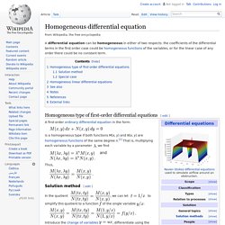
This implies it has scale invariance. When the vector spaces involved are over the real numbers, a slightly less general form of homogeneity is often used, requiring only that (1) hold for all α > 0. Examples[edit] A homogeneous function is not necessarily continuous, as shown by this example. Function (mathematics) A function f takes an input x, and returns a single output f(x).
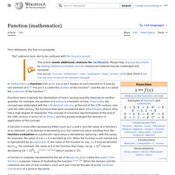
One metaphor describes the function as a "machine" or "black box" that for each input returns a corresponding output. One Grain of Rice. The following excerpt is taken from the book One Grain of Rice by Demi.

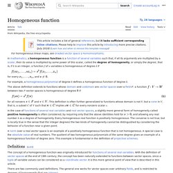
(If you do not have access to this book, consider telling students a similar story as a way of introducing the lesson. This will also provide the background needed for writing algebraic equations, as well as the other mathematical details of the lesson. When using this lesson plan, simply skip the parts that indicate which pages of the book to read aloud, but note that you can still ask the same questions.) Long ago in India, there lived a raja who believed that he was wise and fair. But every year he kept nearly all of the people’s rice for himself. Taylor series. As the degree of the Taylor polynomial rises, it approaches the correct function.
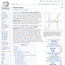
This image shows sin(x) and its Taylor approximations, polynomials of degree 1, 3, 5, 7, 9, 11 and 13. The exponential functionex (in blue), and the sum of the first n+1 terms of its Taylor series at 0 (in red). A function can be approximated by using a finite number of terms of its Taylor series. Taylor's theorem gives quantitative estimates on the error introduced by the use of such an approximation. Stiff equation. In mathematics, a stiff equation is a differential equation for which certain numerical methods for solving the equation are numerically unstable, unless the step size is taken to be extremely small.
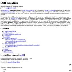
It has proven difficult to formulate a precise definition of stiffness, but the main idea is that the equation includes some terms that can lead to rapid variation in the solution. When integrating a differential equation numerically, one would expect the requisite step size to be relatively small in a region where the solution curve displays much variation and to be relatively large where the solution curve straightens out to approach a line with slope nearly zero.
For some problems this is not the case. Sometimes the step size is forced down to an unacceptably small level in a region where the solution curve is very smooth. The phenomenon being exhibited here is known as stiffness. Louis Bachelier. "Bachelier" redirects here.

For the artist, see Jean-Jacques Bachelier. Louis Jean-Baptiste Alphonse Bachelier (March 11, 1870 – April 28, 1946)[1] was a French mathematician at the turn of the 20th century. The Midas Formula - Stock Market Documentary. Parametric Representation of the Solution Set to a Linear Equation. Fluctuation-dissipation theorem. The fluctuation-dissipation theorem (FDT) is a powerful tool in statistical physics for predicting the behavior of systems that obey detailed balance.
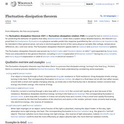
Given that a system obeys detailed balance, the theorem is a general proof that thermal fluctuations in a physical variable predict the response quantified by the admittance or impedance of the same physical variable, and vice versa. The fluctuation-dissipation theorem applies both to classical and quantum mechanical systems. The fluctuation-dissipation theorem relies on the assumption that the response of a system in thermodynamic equilibrium to a small applied force is the same as its response to a spontaneous fluctuation. Therefore, the theorem connects the linear response relaxation of a system from a prepared non-equilibrium state to its statistical fluctuation properties in equilibrium.[1] Often the linear response takes the form of one or more exponential decays. Qualitative overview and examples[edit] Resistance and Johnson noise. Parametric Form of a System Solution. We now know that systems can have either no solution, a unique solution, or an infinite solution.
Moreover, the infinite solution has a specific dimension dependening on how the system is constrained by independent equations. The nature of the solution of systems used previously has been somewhat obvious due to the limited number of variables and equations used. In real-life practice, many hundreds of equations and variables may be needed to specify a system. As they have done before, matrix operations allow a very systematic approach to be applied to determine the nature of a system's solution. GeoGebra. GCSE Maths and English Revision Videos. Laplacian Equations. Math. Practical solution to any problem. Wallpaper group. Wallpaper groups are two-dimensional symmetry groups, intermediate in complexity between the simpler frieze groups and the three-dimensional crystallographic groups (also called space groups). Introduction[edit] Wallpaper groups categorize patterns by their symmetries.
Subtle differences may place similar patterns in different groups, while patterns that are very different in style, color, scale or orientation may belong to the same group. State-Space Analysis of Time-Varying Higher-Order Spike Correlation for Multiple Neural Spike Train Data. Results General formulation Log-linear model of multiple neural spike sequences. We consider an ensemble spike pattern of. Calculating with Time. Even otherwise highly numerate people have been known to throw up their hands in horror at the thought of adding together times.
A system like time, which is not decimal, can be counter-intuitive and requires concentration. However, with a bit of application, you too can learn how to calculate with time, and gain confidence in manipulating hours, minutes and seconds. Basic Units of Time The basic units of time, which allow you to do calculations involving time, are: Years are commonly split into quarters, especially in business and education settings with each quarter being three months or approximately 90 days. Cauchy–Riemann equations. Holomorphic function. A rectangular grid (top) and its image under a conformal map f (bottom). Seeing the S-curve in everything. Esses are everywhere. Demonstrating the importance of dynamical systems theory. Two new papers demonstrate the successes of using bifurcation theory and dynamical systems approaches to solve biological puzzles. Predicting burglary patterns through math modeling of crime. Pattern formation in physical, biological, and sociological systems has been studied for many years.
How the zebra gets its stripes: A simple genetic circuit. Many living things have stripes, but the developmental processes that create these and other patterns are complex and difficult to untangle. A Few of My Favorite Spaces: The Topologist's Sine Curve - Roots of Unity - Scientific American Blog Network. There are four basic properties of sets that beginning analysis and topology students see: open, closed, compact, and connected. Uber, but for Topological Spaces - Roots of Unity - Scientific American Blog Network.
So it’s cold and rainy, and you’re up a little too late trying to figure out why that one pesky assumption is necessary in a theorem. Wouldn’t it be nice if you could just order up a space that was path connected but not locally connected? You’re in luck, there’s an app a website for that. The π-Base will deliver an Alexandroff Square right to your door computer screen. Davide P. Cervone (Math/Pythagorus): Pythagorian Theorem. 4th Dimension Cube-flatland: Cubes Fall Through Flatland. From Wolfram MathWorld. A dissection fallacy is an apparent paradox arising when two plane figures with different areas seem to be composed by the same finite set of parts. In order to produce this illusion, the pieces have to be cut and reassembled so skillfully, that the missing or exceeding area is hidden by tiny, negligible imperfections of shape.
Fibonacci Numbers and The Golden Section in Art, Architecture and Music. The Golden Section - the Number and Its Geometry. The Mathematical Magic of the Fibonacci Numbers. GeoGebra. Visually stunning math concepts which are easy to explain. Prime Number Theorem: the density of primes (Prime Adventure part 6) Untitled.
Untitled. Untitled. Untitled. Untitled. Untitled. 3 Solved Math Mysteries (and 2 That Still Plague Us) Untitled. A Trigonometric Trip Through Time - Introduction. 21 GIFs That Explain Mathematical Concepts. Visually stunning math concepts which are easy to explain. 21 GIFs That Explain Mathematical Concepts. Math. Vedic math.