
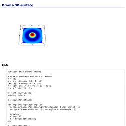
Gnuplot Version 4.6 SVG terminal demos. Gnuplot demo script: surface1.dem. Gnuplot demo script: surface1.dem. Yapso, Yet Another Plotting System for Octave. Draw a 3D-surface Code function anim_camera(fname) % draw a sombrero and turn it around n = 50; x = y = linspace (-8, 8, n)'; [xx, yy] = meshgrid (x, y); r = sqrt (xx .^ 2 + yy .^ 2) + eps; c = 5 * sin (r) ./ r; h= surf(xx,yy,c,c); shading interp m = moviefile(fname); for angle=linspace(0,2*pi,50) set(gca,'CameraPosition',20*[sin(angle) 0 cos(angle) ]); set(gca,'CameraUpVector',[-cos(angle) 0 sin(angle) ]); drawnow sleep(.01) m = movieaddframe(m); end m = movieclose(m); Download anim_camera.m Draw several curves with different styles title('Some line propeties'); x = 0:0.1:6; hold on plot(x,sin(x),'b'); plot(x,sin(x-.4),'ro'); plot(x,sin(x-.8),'g--'); plot(x,sin(x-1.2),'c+'); hold off Download test_plot.m Draw the GNU Octave logo.
Output terminals « Gnuplotting. April 27th, 2010 | 50 Comments Gnuplot gives us the opportunity to produce great looking plots in a lot of different formats.
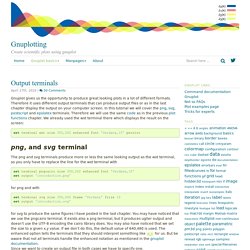
Therefore it uses different output terminals that can produce output files or as in the last chapter display the output on your computer screen. In this tutorial we will cover the png, svg, postscript and epslatex terminals. Therefore we will use the same code as in the previous plot functions chapter. We already used the wxt terminal there which displays the result on the screen: set terminal wxt size 350,262 enhanced font 'Verdana,10' persist png, and svg terminal The png and svg terminals produce more or less the same looking output as the wxt terminal, so you only have to replace the line for the wxt terminal with set terminal pngcairo size 350,262 enhanced font 'Verdana,10'set output 'introduction.png' for png and with set terminal svg size 350,262 fname 'Verdana' fsize 10set output 'introduction.svg' postscript terminal Finally, we will get the following figure.
Gnuplot demo script: histograms.dem. GNUplot: część 12. - Ustawienia legendy - Świat komputerów, porady i rozwiązania. Mateusz Chmielewski, 23:42 sobota, 12.02.2011 r.
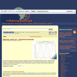
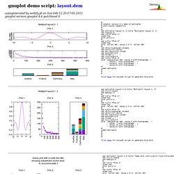
W tej części poradnika do programu GNUplot chciałbym poruszyć temat ustawień legendy wykresu - bardzo ważnego elementu rzutującego na klarowność odbioru zestawionych danych. Z tego powodu niezbędna jest umiejętność jej modyfikacji do konkretnych przypadków i potrzeb. Pokażę zatem między innymi jak zmienić położenie legendy, czy orientację danych, które zawiera. 1. Włączanie i wyłączanie legendy Legenda wykresu w programie GNUplot jest włączona w sposób domyślny, więc o ile wcześniej sami jej nie wyłączyliśmy, będzie widoczna. Set key off; W ten sposób legenda całkowicie zniknie z obszaru wykresu. Gnuplot demo script: layout.dem. # # Stacked Plot Demo # # Set top and bottom margins to 0 so that there is no space between plots. # Fix left and right margins to make sure that the alignment is perfect. # Turn off xtics for all plots except the bottom one. # In order to leave room for axis and tic labels underneath, we ask for # a 4-plot layout but only use the top 3 slots. # set tmargin 0 set bmargin 0 set lmargin 3 set rmargin 3 unset xtics unset ytics set multiplot layout 4,1 title "Auto-layout of stacked plots\n" set key autotitle column nobox samplen 1 noenhanced unset title set style data boxes set yrange [0 : 800000] plot 'immigration.dat' using 3 lt 1 plot 'immigration.dat' using 8 lt 3 set xtics nomirror set tics scale 0 font ",8" set xlabel "Immigration to U.S. by Decade" plot 'immigration.dat' using 21:xtic(1) lt 4 unset multiplot Click here for minimal script to generate this plot.
Gnuplotting. Gnuplot tricks.