
CSS and R markdown. Custom CSS for HTML generated using RStudio. People have been telling me for a while that the latest version of RStudio, the IDE for R, is a great way to generate reports.
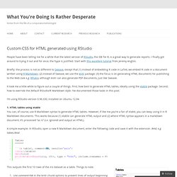
I finally got around to trying it out and for once, the hype is justified. Start with this excellent tutorial from Jeremy Anglim. Briefly: the process is not so different to Sweave, except that (1) instead of embedding R code in LaTeX, we embed R code in a document written using R Markdown; (2) instead of Sweave, we use the knitr package; (3) the focus is on generating HTML documents for publishing to the Web (see e.g. RPubs), although knitr can also generate PDF documents, just like Sweave. It took me a little while to figure out a couple of things. 1. A simple example. A simple table using xtable + R Markdown This outputs the first 10 rows of the iris dataset as a table.
(update: comment=NA is redundant here; see the helpful comment from Yihui at end of post) 2. The table with custom CSS applied.
Writing papers using R Markdown. I have been watching the activity in RStudio and knitr for a while, and have even been using Rmd (R markdown) files in my own work as a way to easily provide commentary on an actual dataset analysis.
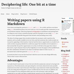
Yihui has proposed writing papers in markdown and posting them to a blog as a way to host a statistics journal, and lots of people are now using knitr as a way to create reproducible blog posts that include code (including yours truly). The idea of writing a paper that actually includes the necessary code to perform the analysis, and is actually readable in its raw form, and that someone else could actually run was pretty appealing. Unfortunately, I had not had the time or opportunity to actually try it, until recently our group submitted a conference paper that included a lot of analysis in R that seemed like the perfect opportunity to try this. (I will link to the paper here when I hear more, or get clearance from my PI). Advantages Tables and Figures Counting ## _ t.blogPostDocs ## 0 1. Markdown Syntax Documentation. Note: This document is itself written using Markdown; you can see the source for it by adding ‘.text’ to the URL.
Overview Philosophy Markdown is intended to be as easy-to-read and easy-to-write as is feasible. Readability, however, is emphasized above all else. A Markdown-formatted document should be publishable as-is, as plain text, without looking like it’s been marked up with tags or formatting instructions. To this end, Markdown’s syntax is comprised entirely of punctuation characters, which punctuation characters have been carefully chosen so as to look like what they mean. Inline HTML. Installing old R package versions. A big problem in reproducible research is that software changes.
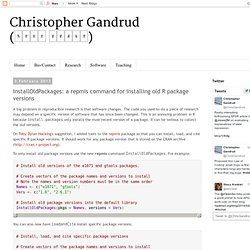
The code you used to do a piece of research may depend on a specific version of software that has since been changed. This is an annoying problem in R because install.packages only installs the most recent version of a package. It can be tedious to collect the old versions. On Toby Dylan Hocking's suggestion, I added tools to the repmis package so that you can install, load, and cite specific R package versions. It should work for any package version that is stored on the CRAN archive ( To only install old package versions use the new repmis command InstallOldPackages. . # Install old versions of the e1071 and gtools packages. # Create vectors of the package names and versions to install# Note the names and version numbers must be in the same orderNames <- c("e1071", "gtools")Vers <- c("1.6", "2.6.1") # Install old package versions into the default libraryInstallOldPackages(pkgs = Names, versions = Vers)
Getting Started with R Markdown, knitr, and Rstudio 0.96. This post examines the features of R Markdown using knitr in Rstudio 0.96.
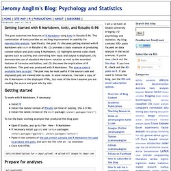
This combination of tools provides an exciting improvement in usability for reproducible analysis. Testing R Markdown with R Studio and posting it on RPubs.com. How to Convert Sweave LaTeX to knitr R Markdown: Winter Olympic Medals Example. The following post shows how to manually convert a Sweave LaTeX document into a knitr R Markdown document.
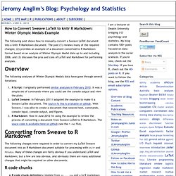
The post (1) reviews many of the required changes; (2) provides an example of a document converted to R Markdown format based on an analysis of Winter Olympic Medal data up to and including 2006; and (3) discusses the pros and cons of LaTeX and Markdown for performing analyses. The following analyses of Winter Olympic Medals data have gone through several iterations: R Script: I originally performed similar analyses in February 2010. It was a simple set of commands where you could see the console output and view the plots. Splitting and Combining R pdf Graphics. Interactive reports in R with knitr and RStudio. Citations in markdown using knitr. I am finding myself more and more drawn to markdown rather then tex/Rnw as my standard format (not least of which is the ease of displaying the files on github, particularly now that we have automatic image uploading).
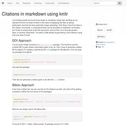
One thing I miss from latex is the citation commands. (I understand these can be provided to markdown via Pandoc, but I’d like to simply have to knit the document, and not then run it through pandoc, latex, or another interpreter). I’ve taken a little whack at generating in-text citations using knitr and other R tools. DOI Approach I’ve put some simple functions in a knitcitations package. Library(devtools) install_github("knitcitations", "cboettig") and load the package require(knitcitations) Then we can generate a citation given a doi with the ref function: Bibtex Approach If we have a bibtex file, we can use this for the citations as well. Library(bibtex) write.bib(c('bibtex', 'knitr', 'knitcitations'), file="example.bib") Now we can simply read in the bibtex files: