
Growing self-organizing map. Self-organizing map. A self-organizing map (SOM) or self-organizing feature map (SOFM) is a type of artificial neural network (ANN) that is trained using unsupervised learning to produce a low-dimensional (typically two-dimensional), discretized representation of the input space of the training samples, called a map.
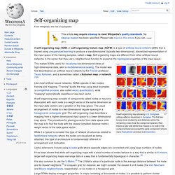
Self-organizing maps are different from other artificial neural networks in the sense that they use a neighborhood function to preserve the topological properties of the input space. This makes SOMs useful for visualizing low-dimensional views of high-dimensional data, akin to multidimensional scaling. The model was first described as an artificial neural network by the Finnish professor Teuvo Kohonen, and is sometimes called a Kohonen map or network.[1][2] Like most artificial neural networks, SOMs operate in two modes: training and mapping. A self-organizing map consists of components called nodes or neurons. Large SOMs display emergent properties. Learning algorithm[edit] Variables[edit] Www.multivu.com/assets/58095/documents/Data-is-the-new-oil-Infographic-original.pdf?utm_source=socialhub&utm_medium=6341&utm_content=5111444572402834168&utm_campaign=
Singular Value Decomposition of a Matrix. Description Compute the singular-value decomposition of a rectangular matrix.

Usage svd(x, nu = min(n, p), nv = min(n, p), LINPACK = FALSE) La.svd(x, nu = min(n, p), nv = min(n, p)) Arguments Details. Astro.rit.edu/~ejipci/Reports/svd.pdf. Www.ling.ohio-state.edu/~kbaker/pubs/Singular_Value_Decomposition_Tutorial.pdf. Singular Value Decomposition. Singular value decomposition. Visualization of the SVD of a two-dimensional, real shearing matrixM.
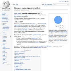
First, we see the unit disc in blue together with the two canonical unit vectors. We then see the action of M, which distorts the disk to an ellipse. The SVD decomposes M into three simple transformations: an initial rotationV*, a scaling Σ along the coordinate axes, and a final rotation U. Www.bioconductor.org/help/course-materials/2003/Milan/Lectures/anestisMilan4.pdf. Www.stanford.edu/group/mmds/slides/li-mmds.pdf. Multifactor dimensionality reduction.
The basis of the MDR method is a constructive induction algorithm that converts two or more variables or attributes to a single attribute.

This process of constructing a new attribute changes the representation space of the data. The end goal is to create or discover a representation that facilitates the detection of nonlinear or nonadditive interactions among the attributes such that prediction of the class variable is improved over that of the original representation of the data. Illustrative example[edit] Consider the following simple example using the exclusive OR (XOR) function. XOR is a logical operator that is commonly used in data mining and machine learning as an example of a function that is not linearly separable. Table 1 A data mining algorithm would need to discover or approximate the XOR function in order to accurately predict Y using information about X1 and X2.
Table 2 The data mining algorithm now has much less work to do to find a good predictive function. Software[edit] Nonlinear dimensionality reduction. High-dimensional data, meaning data that requires more than two or three dimensions to represent, can be difficult to interpret.
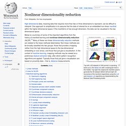
One approach to simplification is to assume that the data of interest lie on an embedded non-linear manifold within the higher-dimensional space. If the manifold is of low enough dimension, the data can be visualised in the low dimensional space. Top-left: a 3D dataset of 1000 points in a spiraling band (a.k.a. the Swiss roll) with a rectangular hole in the middle. Top-right: the original 2D manifold used to generate the 3D dataset. Bottom left and right: 2D recoveries of the manifold respectively using the LLE and Hessian LLE algorithms as implemented by the Modular Data Processing toolkit.
Below is a summary of some of the important algorithms from the history of manifold learning and nonlinear dimensionality reduction (NLDR).[1] Many of these non-linear dimensionality reduction methods are related to the linear methods listed below. Linear methods[edit] Deconstructing Recommender Systems. Photo-illustration: Christina Beard One morning in April, we each directed our browsers to Amazon.com’s website.
Not only did the site greet us by name, the home page opened with a host of suggested purchases. It directed Joe to Barry Greenstein’s Ace on the River: An Advanced Poker Guide, Jonah Lehrer’s Imagine: How Creativity Works, and Michael Lewis’s Boomerang: Travels in the New Third World. For John it selected Dave Barry’s Only Travel Guide You’ll Ever Need, the spy novel Mission to Paris, by Alan Furst, and the banking exposé The Big Short: Inside the Doomsday Machine, also by Michael Lewis. By now, online shoppers are accustomed to getting these personalized suggestions. All of these suggestions come from recommender systems. Over the years, recommenders have evolved considerably. The two of us have been building and studying recommender systems since their early days, initially as academic researchers working on the GroupLens Project. It’s a pretty cool solution.