
Fitting a sigmoid curve in R - Kyriakos Chatzidimitriou. Posted by kyrcha on Jul 8, 2012 in R, Tutorials | 19 Comments This is a short tutorial on how to fit data points that look like a sigmoid curve using the nls function in R.
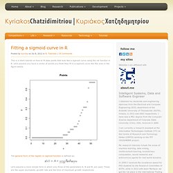
Let’s assume you have a vector of points you think they fit in a sigmoid curve like the ones in the figure below. The general form of the logistic or sigmoid function is defined as: Let’s assume a more simple form in which only three of the parameters K, B and M, are used. Those are the upper asymptote, growth rate and the time of maximum growth respectively. An Introduction to Sphericity. An introduction to sphericity The article is written for a general audience of post-graduate and graduate researchers.
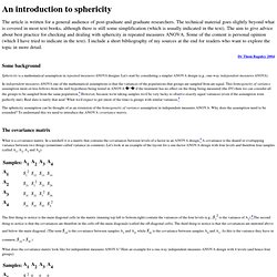
The technical material goes slightly beyond what is covered in most text books, although there is still some simplification (which is usually indicated in the text). The aim to give advice about best practice for checking and dealing with sphericity in repeated measures ANOVA. Some of the content is personal opinion (which I have tried to indicate in the text). I include a short bibliography of my sources at the end for readers who want to explore the topic in more detail. Dr Thom Baguley 2004 Some background Sphericity is a mathematical assumption in repeated measures ANOVA designs.
In independent measures ANOVA one of the mathematical assumptions is that the variances of the populations that groups are sampled from are equal. The sphericity assumption can be thought of as an extension of the homogeneity of variance assumption in independent measures ANOVA. An example. 4.5 - Exponential and Logarithmic Models. Exponential Growth Function y = C ekt, k > 0 Features Asymptotic to y = 0 to left Passes through (0,C) C is the initial value Increases without bound to right Notes Some of the things that exponential growth is used to model include population growth, bacterial growth, and compound interest.
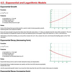
If you are lucky enough to be given the initial value, that is the value when x = 0, then you already know the value of the constant C. Alternatively, almost like cheating, you can put the x-values into List 1, the y-values into List 2, and choose the ExpReg option on the TI-82 calculator. Exponential Decay (decreasing form) y = C e-kt, k > 0 Asymptotic to y = 0 to right Passes through (0,C) C is the initial value Decreasing, but bounded below by y=0 Exponential decay and be used to model radioactive decay and depreciation.
Exponential decay models decrease very rapidly, and then level off to become asymptotic towards the x-axis. Exploratory Data Analysis and Regression in R. Exploratory Data Analysis (EDA) and Regression This tutorial demonstrates some of the capabilities of R for exploring relationships among two (or more) quantitative variables.
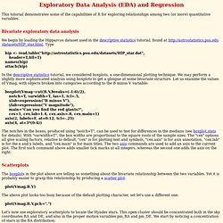
Bivariate exploratory data analysis We begin by loading the Hipparcos dataset used in the descriptive statistics tutorial, found at Type hip <- read.table(" header=T,fill=T) names(hip) attach(hip) In the descriptive statistics tutorial, we considered boxplots, a one-dimensional plotting technique. Boxplot(Vmag~cut(B.V,breaks=(-1:6)/2), notch=T, varwidth=T, las=1, tcl=.5, xlab=expression("B minus V"), ylab=expression("V magnitude"), main="Can you find the red giants?
" The notches in the boxes, produced using "notch=T", can be used to test for differences in the medians (see boxplot.stats for details). Scatterplots The boxplots in the plot above are telling us something about the bivariate relationship between the two variables. Plot(Vmag,B.V)
Exponential Rise to Maximum-www.kxcad.com. Mersenne prime. In mathematics, a Mersenne prime is a prime number of the form .
They are named after the French monk Marin Mersenne who studied them in the early 17th century. The first four Mersenne primes are 3, 7, 31 and 127. If n is a composite number then so is 2n − 1. The definition is therefore unchanged when written where p is assumed prime. More generally, numbers of the form without the primality requirement are called Mersenne numbers. As of February 2014[ref], 48 Mersenne primes are known. About Mersenne primes[edit] Many fundamental questions about Mersenne primes remain unresolved. The first four Mersenne primes are M2 = 3, M3 = 7, M5 = 31 and M7 = 127. A basic theorem about Mersenne numbers states that if Mp is prime, then the exponent p must also be prime. This rules out primality for Mersenne numbers with composite exponent, such as M4 = 24 − 1 = 15 = 3×5 = (22 − 1)×(1 + 22). Though it was believed by early mathematicians that Mp is prime for all primes p, Mp is very rarely prime.