
Quicksort. History[edit] The quicksort algorithm was developed in 1960 by Tony Hoare while in the Soviet Union, as a visiting student at Moscow State University.
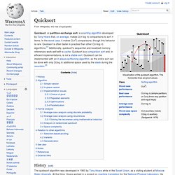
At that time, Hoare worked in a project on machine translation for the National Physical Laboratory. He developed the algorithm in order to sort the words to be translated, to make them more easily matched to an already-sorted Russian-to-English dictionary that was stored on magnetic tape.[3] Algorithm[edit] Full example of quicksort on a random set of numbers. Dijkstra's algorithm. The algorithm exists in many variants; Dijkstra's original variant found the shortest path between two nodes,[3] but a more common variant fixes a single node as the "source" node and finds shortest paths from the source to all other nodes in the graph, producing a shortest-path tree.
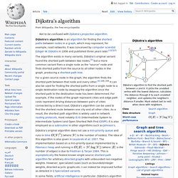
For a given source node in the graph, the algorithm finds the shortest path between that node and every other.[4]:196–206 It can also be used for finding the shortest paths from a single node to a single destination node by stopping the algorithm once the shortest path to the destination node has been determined. For example, if the nodes of the graph represent cities and edge path costs represent driving distances between pairs of cities connected by a direct road, Dijkstra's algorithm can be used to find the shortest route between one city and all other cities. Dijkstra's original algorithm does not use a min-priority queue and runs in time (where is the number of nodes). Prim's algorithm. Prim's algorithm starting at vertex A.
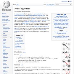
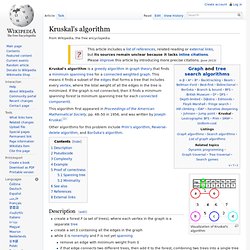
In the second step, BD is chosen to add to the tree instead of AB arbitrarily, as both have weight 2. Afterwards, AB is excluded because it is between two nodes that are already in the tree. Kruskal's algorithm. Visualization of Kruskal's algorithm This algorithm first appeared in Proceedings of the American Mathematical Society, pp. 48–50 in 1956, and was written by Joseph Kruskal.[1]
Sequence alignment. A sequence alignment, produced by ClustalW, of two humanzinc finger proteins, identified on the left by GenBank accession number.
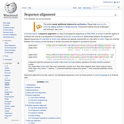
Key: Single letters: amino acids. Red: small, hydrophobic, aromatic, not Y. Blue: acidic. Magenta: basic. Green: hydroxyl, amine, amide, basic. Sequence alignments are also used for non-biological sequences, such as those present in natural language or in financial data. Interpretation[edit] Alignment methods[edit] Very short or very similar sequences can be aligned by hand.
Representations[edit] Sequence alignments can be stored in a wide variety of text-based file formats, many of which were originally developed in conjunction with a specific alignment program or implementation. Global and local alignments[edit] Illustration of global and local alignments demonstrating the 'gappy' quality of global alignments that can occur if sequences are insufficiently similar. Optimal binary search tree. In computer science, an optimal binary search tree (BST) is a binary search tree which provides the smallest possible search time (or expected search time) for a given sequence of accesses (or access probabilities).
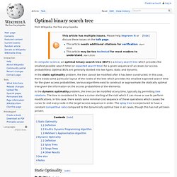
Optimal BSTs are generally divided into two types: static and dynamic. Bellman–Ford algorithm. Algorithm[edit] In this example graph, assuming that A is the source and edges are processed in the worst order, from right to left, it requires the full |V|−1 or 4 iterations for the distance estimates to converge.
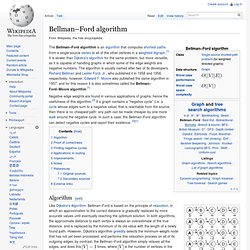
Conversely, if the edges are processed in the best order, from left to right, the algorithm converges in a single iteration. times, where. Floyd–Warshall algorithm. .
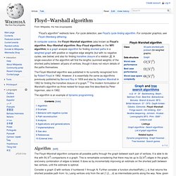
Johnson's algorithm. Topological sorting. Examples[edit] The canonical application of topological sorting (topological order) is in scheduling a sequence of jobs or tasks based on their dependencies; topological sorting algorithms were first studied in the early 1960s in the context of the PERT technique for scheduling in project management (Jarnagin 1960).
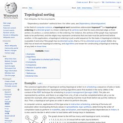
The jobs are represented by vertices, and there is an edge from x to y if job x must be completed before job y can be started (for example, when washing clothes, the washing machine must finish before we put the clothes to dry). Then, a topological sort gives an order in which to perform the jobs. Simplex algorithm. Algorithm History[edit] George Dantzig worked on planning methods for the US Army Air Force during World War II using a desk calculator.
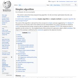
During 1946 his colleague challenged him to mechanize the planning process to distract him from taking another job. Dantzig formulated the problem as linear inequalities inspired by the work of Wassily Leontief, however, at that time he didn't include an objective as part of his formulation. Without an objective, a vast number of solutions can be feasible, and therefore to find the "best" feasible solution, military-specified "ground rules" must be used that describe how goals can be achieved as opposed to specifying a goal itself.
After Dantzig included an objective function as part of his formulation during mid-1947, the problem was mathematically more tractable.