
Wahrscheinlichkeitsverteilung. Die Wahrscheinlichkeitsverteilung, häufig kurz Verteilung, ist ein Begriff der Wahrscheinlichkeitstheorie, der auch in der Mathematischen Statistik eine zentrale Bedeutung besitzt.
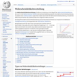
Eine Wahrscheinlichkeitsverteilung ist jeweils einer Zufallsvariablen zugeordnet. Dabei beschreibt die Wahrscheinlichkeitsverteilung, mit welchen Wahrscheinlichkeiten die Zufallsvariable ihre möglichen Werte annimmt. Der Begriff der Wahrscheinlichkeitsverteilung ist das theoretische Pendant zur empirisch ermittelbaren Häufigkeitsverteilung, die Gegenstand der deskriptiven Statistik ist. Verteilung (grün) und Verteilungsfunktion (rot) beim Wurf eines symmetrischen Würfels Beispielsweise wird der Wurf eines symmetrischen Würfels dadurch beschrieben, dass jedes der sechs möglichen Ergebnisse 1, 2, ..., 6 mit der Wahrscheinlichkeit 1/6 eintritt.
Typen von Wahrscheinlichkeitsverteilungen[Bearbeiten] Diskrete Verteilungen[Bearbeiten] Verteilungsfunktion einer diskreten Verteilung angibt. Lévy process. The most well known examples of Lévy processes are Brownian motion and the Poisson process.
Aside from Brownian motion with drift, all other Lévy processes, except the deterministic case, have discontinuous paths. Mathematical definition[edit] A stochastic process. Cauchy distribution. Stable distribution. The importance of stable probability distributions is that they are "attractors" for properly normed sums of independent and identically-distributed (iid) random variables.

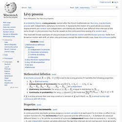
The normal distribution is one family of stable distributions. By the classical central limit theorem the properly normed sum of a set of random variables, each with finite variance, will tend towards a normal distribution as the number of variables increases. Without the finite variance assumption the limit may be a stable distribution. Stable distributions that are non-normal are often called stable Paretian distributions,[citation needed] after Vilfredo Pareto. Lévy distribution. Definition[edit] The probability density function of the Lévy distribution over the domain is where is the location parameter and is the scale parameter.
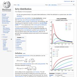
Zeta distribution. In probability theory and statistics, the zeta distribution is a discrete probability distribution.
If X is a zeta-distributed random variable with parameter s, then the probability that X takes the integer value k is given by the probability mass function. Zeta-Verteilung. Zeta-Verteilung mit verschiedenen Parameterwerten von s Die Zeta-Verteilung (auch Zipf-Verteilung nach George Kingsley Zipf) ist eine diskrete Wahrscheinlichkeitsverteilung, die den natürlichen Zahlen x=1,2,3,... die Wahrscheinlichkeiten zuordnet, wobei s>1 ein Parameter und ζ(s) die riemannsche Zetafunktion ist.
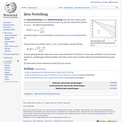
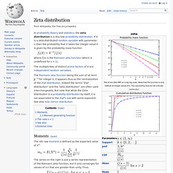
Ihr und liegt in diesem Fall bei Es kann gezeigt werden, dass die Anzahl unterschiedlicher Primfaktoren einer Zeta-verteilten Zufallsvariable wiederum unabhängige Zufallsvariablen sind. Zur Motivation dieser Verteilung siehe Zipfsches Gesetz. Pareto-Verteilung. Die Verteilung der Einwohnerzahlen der 1000 größten deutschen Städte (Histogramm in gelb) kann gut durch eine Pareto-Verteilung (blau) beschrieben werden.
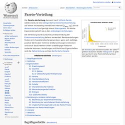
Die Pareto-Verteilung, benannt nach Vilfredo Pareto (1848–1923), ist eine stetige Wahrscheinlichkeitsverteilung auf einem rechtsseitig unendlichen Intervall Die Verteilung wurde zunächst zur Beschreibung der Einkommensverteilung Italiens verwendet. Paretoverteilungen finden sich charakteristischerweise dann, wenn sich zufällige, positive Werte über mehrere Größenordnungen erstrecken und durch das Einwirken vieler unabhängiger Faktoren zustande kommen.
Pareto distribution. The Pareto distribution, named after the Italian civil engineer, economist, and sociologist Vilfredo Pareto, is a power law probability distribution that is used in description of social, scientific, geophysical, actuarial, and many other types of observable phenomena.
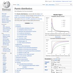
Definition[edit] If X is a random variable with a Pareto (Type I) distribution,[1] then the probability that X is greater than some number x, i.e. the survival function (also called tail function), is given by where xm is the (necessarily positive) minimum possible value of X, and α is a positive parameter. The Pareto Type I distribution is characterized by a scale parameter xm and a shape parameter α, which is known as the tail index. Quasiprobability distribution. A quasiprobability distribution is a mathematical object similar to a probability distribution but which relaxes some of Kolmogorov's axioms of probability theory.
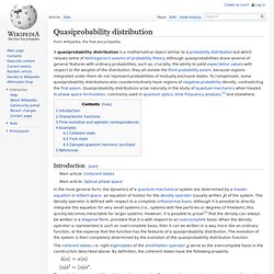
Although quasiprobabilities share several of general features with ordinary probabilities, such as, crucially, the ability to yield expectation values with respect to the weights of the distribution, they all violate the third probability axiom, because regions integrated under them do not represent probabilities of mutually exclusive states. To compensate, some quasiprobability distributions also counterintuitively have regions of negative probability density, contradicting the first axiom. Probability distribution. In applied probability, a probability distribution can be specified in a number of different ways, often chosen for mathematical convenience: A probability distribution can either be univariate or multivariate.
A univariate distribution gives the probabilities of a single random variable taking on various alternative values; a multivariate distribution (a joint probability distribution) gives the probabilities of a random vector—a set of two or more random variables—taking on various combinations of values. List of probability distributions.
Many probability distributions are so important in theory or applications that they have been given specific names. Discrete distributions[edit] With finite support[edit] With infinite support[edit] Beta distribution. In probability theory and statistics, the beta distribution is a family of continuous probability distributions defined on the interval [0, 1] parametrized by two positive shape parameters, denoted by α and β, that appear as exponents of the random variable and control the shape of the distribution. The beta distribution has been applied to model the behavior of random variables limited to intervals of finite length in a wide variety of disciplines.
For example, it has been used as a statistical description of allele frequencies in population genetics;[1] time allocation in project management / control systems;[2] sunshine data;[3] variability of soil properties;[4] proportions of the minerals in rocks in stratigraphy;[5] and heterogeneity in the probability of HIV transmission.[6] Pearson distribution. Diagram of the Pearson system, showing distributions of types I, III, VI, V, and IV in terms of β1 (squared skewness) and β2 (traditional kurtosis) The Pearson distribution is a family of continuous probability distributions.
It was first published by Karl Pearson in 1895 and subsequently extended by him in 1901 and 1916 in a series of articles on biostatistics. History[edit] Rhind (1909, pp. 430–432) devised a simple way of visualizing the parameter space of the Pearson system, which was subsequently adopted by Pearson (1916, plate 1 and pp. 430ff., 448ff.). The Pearson types are characterized by two quantities, commonly referred to as β1 and β2. Where γ1 is the skewness, or third standardized moment.
Many of the skewed and/or non-mesokurtic distributions familiar to us today were still unknown in the early 1890s. Definition[edit] A Pearson density p is defined to be any valid solution to the differential equation (cf. With : follows directly from the differential equation. and. Q-Gaussian distribution. The q-Gaussian has been applied to problems in the fields of statistical mechanics, geology, anatomy, astronomy, economics, finance, and machine learning.
The distribution is often favored for its heavy tails in comparison to the Gaussian for . There is generalized q-analog of the classical central limit theorem[2] in which the independence constraint for the i.i.d. variables is relaxed to an extent defined by the q parameter, with independence being recovered as q → 1. In analogy to the classical central limit theorem, an average of such random variables with fixed mean and variance tend towards the q-Gaussian distribution. Gaussian q-distribution. The distribution is symmetric about zero and is bounded, except for the limiting case of the normal distribution. The limiting uniform distribution is on the range -1 to +1. Definition[edit] The Gaussian q-density. Matrix normal distribution. In statistics, the matrix normal distribution is a probability distribution that is a generalization of the multivariate normal distribution to matrix-valued random variables. Definition[edit] The probability density function for the random matrix X (n × p) that follows the matrix normal distribution has the form: where M is n × p, U is n × n and V is p × p.
There are several ways to define the two covariance matrices. Where is a constant which depends on U and ensures appropriate power normalization. Complex normal distribution. In probability theory, the family of complex normal distributions characterizes complex random variables whose real and imaginary parts are jointly normal,[1] i.e., normally distributed and independent.
The complex normal family has three parameters: location parameter μ, covariance matrix Γ, and the relation matrix C. The standard complex normal is the univariate distribution with μ = 0, Γ = 1, and C = 0. An important subclass of complex normal family is called the circularly-symmetric complex normal and corresponds to the case of zero relation matrix and zero mean: .[2] Circular symmetric complex normal random variables are used extensively in signal processing, and are sometimes referred to as just complex normal in signal processing literature. Definition[edit] Suppose X and Y are random vectors in Rk such that vec[X Y] is a 2k-dimensional normal random vector. Rectified Gaussian distribution. Distribution (Mathematik) Eine Distribution bezeichnet im Bereich der Mathematik eine besondere Art eines Funktionals, also ein Objekt aus der Funktionalanalysis. Der Mathematiker Laurent Schwartz war maßgeblich an der Untersuchung der Theorie der Distributionen beteiligt.
Im Jahr 1950 veröffentlichte er den ersten systematischen Zugang zu dieser Theorie. Für seine Arbeiten über die Distributionen erhielt er die Fields-Medaille. Jacques Hadamard Im Jahr 1903 führte Jacques Hadamard den für die Distributionentheorie zentralen Begriff des Funktionals ein. Paul Dirac, 1933 dargestellt werden kann. Delta-Distribution. Definition[Bearbeiten] Der Testfunktionenraum für die Delta-Distribution ist der Raum der beliebig oft differenzierbaren Funktionen mit bzw. offen. Dirac delta function. Schematic representation of the Dirac delta function by a line surmounted by an arrow. Cumulative distribution function. Elliptical distribution. Normal distribution. Hypergeometric distribution. Joint probability distribution. Multivariate stable distribution. Multivariate normal distribution. Negative multinomial distribution. Multinomial distribution.