
Problème de flot maximum. Un article de Wikipédia, l'encyclopédie libre.

Un exemple de graphe de flot avec un flot maximum. la source est , et le puits . Les nombres indiquent le flot et la capacité. Le problème de flot maximum consiste à trouver un flot réalisable depuis une source unique et vers un puits unique graphe de flot qui soit maximum[1]. Définitions et variantes[modifier | modifier le code] Quelquefois le problème répond simplement à la question de trouver la valeur de ce flot. Applications[modifier | modifier le code] Solutions[modifier | modifier le code] Étant donné un graphe orienté , où chaque arête a une capacité , on cherche un flot maximum depuis la source vers le puits , sous contrainte de capacité.
Pour une liste plus complète, voir[1]. Algorithme de Ford-Fulkerson. Un article de Wikipédia, l'encyclopédie libre.

L'algorithme de Ford-Fulkerson, du nom de ses auteurs L. R. Ford et D. R. Fulkerson, consiste en une procédure itérative qui permet de déterminer un flot (ou flux) de valeur maximale (ou minimale) à partir d'un flot constaté. Exemple[modifier | modifier le code] Une société de fret dispose de trois centres : un à Paris, le deuxième à Lyon, le troisième à Marseille. Chacun des centres de fret a une capacité maximale de transport ainsi qu'un stock initial de marchandises. Dans l'exemple présent, la matrice associée porte donc dans sa première colonne les valeurs des dits stocks. Le problème peut être généralisé à une circulation dans un réseau (véhicules, fluides, monnaie, etc).
Maximum flow problem - Wikipedia, the free encyclopedia - Mozill. Push-relabel maximum flow algorithm - Wikipedia, the free encycl. In mathematical optimization, the push–relabel algorithm (alternatively, preflow–push algorithm) is an algorithm for computing maximum flows.

The name "push–relabel" comes from the two basic operations used in the algorithm. Throughout its execution, the algorithm maintains a "preflow" and gradually converts it into a maximum flow by moving flow locally between neighboring vertices using push operations under the guidance of an admissible network maintained by relabel operations. In comparison, the Ford–Fulkerson algorithm performs global augmentations that send flow following paths from the source all the way to the sink.[1] The push–relabel algorithm is considered one of the most efficient maximum flow algorithms. The generic algorithm has a strongly polynomial O(V2E) time complexity, which is asymptotically more efficient than the O(VE2) Edmonds–Karp algorithm.[2] Specific variants of the algorithms achieve even lower time complexities. Push-relabel maximum flow algorithm - Wikipedia, the free encycl. Push-relabel maximum flow algorithm - Wikipedia, the free encycl.
Edmonds-Karp algorithm. In computer science and graph theory, the Edmonds–Karp algorithm is an implementation of the Ford–Fulkerson method for computing the maximum flow in a flow network in O(V E2) time.

The algorithm was first published by Yefim (Chaim) Dinic in 1970[1] and independently published by Jack Edmonds and Richard Karp in 1972.[2] Dinic's algorithm includes additional techniques that reduce the running time to O(V2E). Algorithm[edit] The algorithm is identical to the Ford–Fulkerson algorithm, except that the search order when finding the augmenting path is defined. The path found must be a shortest path that has available capacity. This can be found by a breadth-first search, as we let edges have unit length. Pseudocode[edit] For a more high level description, see Ford–Fulkerson algorithm. algorithm EdmondsKarp input: C[1..n, 1..n] (Capacity matrix) E[1..n, 1..?] Example[edit] Given a network of seven nodes, source A, sink G, and capacities as shown below: In the pairs written on the edges, Linear programming. A pictorial representation of a simple linear program with two variables and six inequalities.
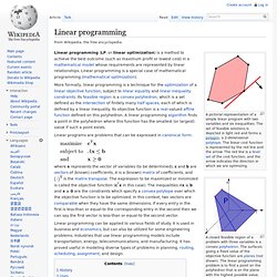
The set of feasible solutions is depicted in light red and forms a polygon, a 2-dimensional polytope. The linear cost function is represented by the red line and the arrow: The red line is a level set of the cost function, and the arrow indicates the direction in which we are optimizing. Linear programming (LP, or linear optimization) is a method to achieve the best outcome (such as maximum profit or lowest cost) in a mathematical model whose requirements are represented by linear relationships.
Linear programming is a special case of mathematical programming (mathematical optimization). Linear programs are problems that can be expressed in canonical form: is the matrix transpose. History[edit] The problem of solving a system of linear inequalities dates back at least as far as Fourier, after whom the method of Fourier–Motzkin elimination is named.